$$\require{color}$$ $$\require{amsmath}$$ $$\require{cancel}$$ $$\definecolor{purple}{RGB}{226, 15, 233}$$ $$\definecolor{grey}{RGB}{177, 159, 149}$$ $$\newcommand{\ii}{\mathbf{i}}$$ $$\newcommand{\parll}{ {\mathbin{\parallel}} }$$ $$\newcommand{\prll}{{\mathbin{\!/\mkern-5mu/\!}}}$$

Topic 3 Applications of Derivatives

3.1 Maxima and Minima

Let \(f\) be a function defined in the domain \(D\) and \(c\) a number in \(D\).

1. We say \(f(c)\) is the absolute maximum value of \(f\) on \(D\) if \(f(c)\geq f(x)\) for all \(x\) in \(D\).
2. We say \(f(c)\) is the absolute minimum value of \(f\) on \(D\) if \(f(c)\leq f(x)\) for all \(x\) in \(D\).
3. We say \(f(c)\) is a local maximum value of \(f\) if \(f(c)\geq f(x)\) for all \(x\) near \(c\).
4. We say \(f(c)\) is a local minimum value of \(f\) if \(f(c)\leq f(x)\) for all \(x\) near \(c\).

Theorem 3.1 (The Extreme Value Theorem) If \(f\) is continuous on a closed interval \([a, b]\), then \(f\) attains an absolute maximum value \(f(c)\) and an absolute minimum value \(f(d)\) at some numbers \(c\) and \(d\) in \([a, b]\).

Theorem 3.2 (Fermat’s Theorem) If \(f\) has a local maximum or minimum at \(c\), and if \(f'(c)\) exists, then \(f'(c)=0\).

A critical value of a function \(f\) is a number \(c\) in its domain such that either \(f'(c)=0\) or \(f'(c)\) does not exist.

How to find the absolute maximum and minimum?

Let \(f\) be function defined over \([a, b]\). To find the absolute maximum and minimum values over \([a,b]\), you may do the following:

1. Find the values of \(f\) at the critical values in \([a, b]\).
2. Find the values of \(f(a)\) and \(f(b)\).
3. The largest of the values from Steps 1 and 2 is the absolute maximum value; the smallest of these values is the absolute minimum value.

Exercise 3.1 Sketch the graph of \(f(x)=\sqrt{x}+1\) and use your sketch to find the absolute and local maximum and minimum values of \(f\) over its domain if they exist.

Solution.

The graph of the function shows that the function \(f\) only has a global minimum \(f(0)=1\).

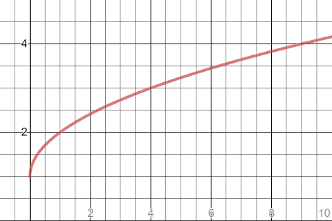
The graph of the function sqrt(x)+1

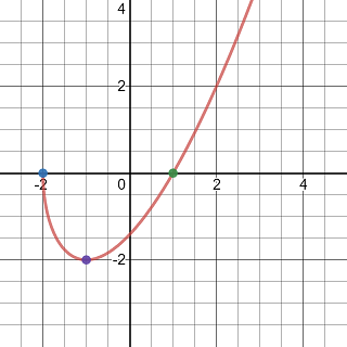
Exercise 3.2 Sketch the graph of \[ f(x)=\begin{cases} \frac12x^{3}+\frac12 & -\frac{3}{2}<x\le 1\\[0.5ex] -x+2 & 1<x<2 \\[0.5ex] \left(x-3\right)^{2}-1 & 2\le x\le 5 \end{cases} \] and use your sketch to find the absolute and local maximum and minimum values of \(f\) over its domain if they exist.

Solution.

The graph of the function shows that the function \(f\) has

1. a global minimum \(f(-\frac32)=-\frac{19}{16}\).
2. a global maximum \(f(5)=3\).
3. a local minimum \(f(3)=-1\).
4. a local maximum \(f(1)=1\).

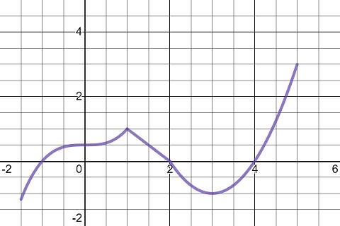
The graph of the function sqrt(x)+1

Exercise 3.3 Find the critical values of the function \(f(x)=2x^3-3x^2-12x\).

Solution.

Find the derivative function first. \[ f'(x)=6x^2-6x-12. \] Because \(f'(x)\) is a polynomial function, it is defined over the whole number line. So the only critical values are the solutions of the equation \(6x^2-6x-12=0\). Solve the equation by factoring, we found that \(x=-1\) or \(x=2\).

The critical values of the \(f\) are \(x=-1\) and \(x=2\).

Exercise 3.4 Find the critical values of the function \(f(x)=\sin x-\cos x\).

Solution.

Find the derivative function first. \[ f'(x)=\cos x+\sin x. \] Because \(f'(x)\) is a polynomial function, it is defined over the whole number line. So the only critical values are the solutions of the equation \(\cos x+\sin x=0\).

To find the solutions, you may rewrite the equation into \(\tan x=-1\) by dividing \(\cos x\) and subtracting 1 from both hand sides. Then \(x=-\frac{\pi}{4}+k\pi\).

The critical values of the \(f\) are \(x=-\frac{\pi}{4}+k\pi\).

Exercise 3.5 Find the critical values of the function \(f(x)=|x^2-2x-3|\).

Solution.

Because an absolute function is not differentiable everywhere. We cannot take the derivative directly. Instead, we should treat the function as a piecewise function by removing the absolute value sign. For that purpose, we have to find intervals where the inside function \(y=x^2-2x-3\) is positive or negative.

Solve the equation \(x^2-2x-3=0\), we found \(x=-1\) or \(x=3\) which are the \(x\)-coordinates of the \(x\)-intercepts of the parabola. As the parabola opens upward, \(x^2-2x-3<0\) only if \(-1<x<3\). So \[ f(x)=|x^2-2x-3| =\begin{cases} -(x^2-2x-3) & -1< x< 3\\[0.5em] x^2-2x-3 & \text{otherwise} \end{cases} \] and the derivative function is \[ f'(x)= \begin{cases} -2x+2 & 1\le x\le 3\\[0.5em] 2x-2 & \text{otherwise} \end{cases} \]

Solving \(f'(x)=0\), we get one critical value \(x=1\). Besides, comparing the left derivatives and right derivatives, we find that \(f'(x)\) is not define at \(x=-1\) or \(x=3\).

So the function \(f\) has three critical values: \(x=-1\), \(x=1\) and \(x=3\).

Exercise 3.6 Find the absolute maximum and absolute minimum values of \(f(x)=x^{3}-3x^{2}-9x+1\) over the interval \([-4, 4]\).

Solution.

To find the absolute maximum and minimum values, we evaluate the function at critical values and endpoints of the interval.

First find the derivative function \[ f'(x)=3x^2-6x-9. \]

Because \(f'\) is continuous. The only critical values are the solutions of the equation. \[ 3x^2-6x-9=0. \]

Solve by factoring, we get the critical values \(x=-1\) and \(x=3\).

Comparing the function values \(f(-4)=-75\), \(f(-1)=6\), \(f(3)=-26\) and \(f(4)=-19\), we know that the absolute maximum value of \(f(x)=x^{3}-3x^{2}-9x+1\) on \([-4, 4]\) is \(f(-1)=6\) and the absolute minimum value of \(f\) on \([-4, 4]\) is \(f(-4)=-75\).

Exercise 3.7 Find the absolute maximum and absolute minimum values of \(f(x)=x+\frac4{x}\) over the interval \([1, 4]\).

Solution.

To find the absolute maximum and minimum values, we evaluate the function at critical values and endpoints of the interval.

First find the derivative function \[ f'(x)=1-\frac{4}{x^2}. \]

Because \(f'\) is continuous on (1, 4). The only critical values are the solutions of the equation. \[ 1-\frac{4}{x^2}=0. \]

Clearing denominator and solving the resulting, we get the critical values \(x=-2\) and \(x=2\). Only \(x=2\) is in the interval \([1.4]\). We only need to compare three values \(f(1)=-3\), \(f(2)=0\) and \(f(4)=3\).

Therefore, the absolute maximum value of \(f(x)=x+\frac4{x}\) on \([1, 4]\) is \(f(4)=3\) and the absolute minimum value of \(f(x)=x+\frac4{x}\) on \([1, 4]\) is \(f(1)=-3\).

Exercise 3.8 Find the absolute maximum and absolute minimum values of \(f(x)=\cos(2x)+2\sin x\) over the interval \([\frac{\pi}{2}, \pi]\).

Solution.

First find the derivative function \[ f'(x)=-2\sin(2x)+2\cos x. \]

Because \(f'\) is continuous. The only critical values are the solutions of the equation. \[ -2\sin(2x)+2\cos x. \]

To solve the equation, we use the double angle formula \(\sin(2x)=2\sin x\cos x\). The equations is then equivalent to \[ -4\sin x\cos x+2\cos x=0. \] Equivalently, \(\cos x=0\) or \(\sin x=\frac12\). Within the interval \([\frac{\pi}{2}, \pi]\), we have solutions \(x=\frac{\pi}{2}\) and \(x=\frac{5\pi}{6}\) which are the critical values.

Because \(f\left(\frac{\pi}{2}\right)=f(\pi)=1\) and \(f\left(\frac{5\pi}{6}\right)=\frac32\). The absolute maximum value of \(f(x)=\cos(2x)+2\sin x\) on \([\frac{\pi}{2}, \pi]\) is \(f\left(\frac{5\pi}{6}\right)=\frac32\) and the absolute minimum value of \(f(x)=\cos(2x)+2\sin x\) on \([\frac{\pi}{2}, \pi]\) is \(f\left(\frac{\pi}{2}\right)=f(\pi)=1\).

Exercise 3.9 Find the absolute maximum and absolute minimum values of \(f(x)=x\sqrt{4x-x^2}\).

Solution.

The domain of the function is determined by \(4x-x^2\geq 0\). Equivalently, \(0\le x\le 4\). We will find absolute extremum values on \([0, 4]\).

First find the derivative function. Apply the product rule and chain rule, we get \[ f'(x)=\sqrt{4x-x^2}+\frac{x(2-x)}{\sqrt{4x-x^2}}. \]

The function is well-defined on \((0, 4)\). So the only critical values are the solutions, in the interval \((0, 4)\), of the equation \[ \sqrt{4x-x^2}+\frac{x(2-x)}{\sqrt{4x-x^2}}=0 \]

Clear denominator and solve, we get a critical value \(x=3\).

Because \(f(0)=f(4)=0\) and \(f(3)=3\sqrt{3}\). The absolute maximum value of \(f(x)=x\sqrt{4x-x^2}\) is \(f(3)=3\sqrt{3}\) and the absolute minimum value of \(f(x)=x\sqrt{4x-x^2}\) is \(f(0)=f(4)=0\).

Exercise 3.10 Find the absolute maximum and absolute minimum values of \(f(x)=|2x^2-x-3|\) over the interval \([-1, 4]\).

Solution.

The absolute value function is now everywhere differentiable. So we first remove the absolute value sign and rewrite the function as a piecewise defined function.

For that purpose, we need to find the interval where \(g(x)=2x^2-x-3\) is negative. Solve the inequality \(2x^2-x-3<0\), we get \(-1<x<\frac32\). Therefore, \[ f(x)=|2x^2-x-3|= \begin{cases} -(2x^2-x-3) & -1<x<\frac32\\[0.5em] 2x^2-x-3 & \frac32\le x\le 4 \end{cases} \]

The derivative function is \[ f'(x)= \begin{cases} -4x+1 & -1<x<\frac32\\[0.5em] 4x-1 & \frac32\le x\le 4 \end{cases} \]

So the function \(f\) has two critical points in \((-1, 4)\): \(x=\frac14\), solved from \(f'(x)=0\), and \(x=\frac32\), where \(f'\) is undefined.

Comparing the values \(f(-1)=0\), \(f\left(\frac14\right)=\frac{25}{8}\), \(f\left(\frac32\right)=0\) and \(f(4)=25\), we know that the absolute maximum value of \(f(x)=|2x^2-x-3|\) on \([-1, 4]\) is \(f(4)=25\) and the absolute minimum value of \(f(x)=|2x^2-x-3|\) on \([-1, 4]\) is \(f(-1)=f\left(\frac32\right)=0\).

3.2 The Mean Value Theorem

The average rate of change is very useful in science and other fields. When a function is differentiable, we even have a better result, the mean value theorem, which is a generalization of the following theorem.

Theorem 3.3 (Role's Theorem) Let \(f\) be a function that satisfies the following three hypotheses:
1. \(f\) is continuous on the closed interval \([a, b]\).
2. \(f\) is differentiable on the open interval \((a, b)\).
3. \(f(a)=f(b)\).
Then there is a number \(c\) in the open interval \((a,b)\) such that \(f'(c)=0\).

Theorem 3.4 (The Mean Value Theorem) Let \(f\) be a function that satisfies the following three hypotheses:
1. \(f\) is continuous on the closed interval \([a, b]\).
2. \(f\) is differentiable on the open interval \((a, b)\).
Then there exists a number \(c\in (a, b)\) such that \[ f'(c)=\frac{f(b)-f(a)}{b-a}, \] equivalently, \[ f(b)-f(a)=f'(c)(b-a). \]

The Mean Value Theorem can be used to show some basic facts in calculus.

Theorem 3.5 If \(f'(x)=0\) for all \(x\) in an interval \((a, b)\), then \(f\) is constant on \((a, b)\).

Corollary 3.1 If \(f'(x)=g'(x)\) for all \(x\) in an interval \((a, b)\), then \(f=g+c\) on \((a, b)\), where \(c\) is a constant number.

Exercise 3.11 Verify that the function \(f(x)=x^2-2x-8\) satisfies the three hypotheses of Rolle’s Theorem over the interval \([-2,4]\) and find all numbers \(c\) in \((-2, 4)\) that satisfy the conclusion of Rolle’s Theorem.

Solution.

As a polynomial function \(f\) is continuous on \([-2, 4]\) and differentiable on \((-2, 4)\). The function has the following values \(f(-2)=0\) and \(f(4)=0\). So Rolle’s theorem can be applied over \([-2, 4]\). To find \(c\) in \((-2, 4)\) satisfying Rolle’s theorem, we solve for \(x\) from the equation \(f'(x)=0\) in the interval \((-2, 4)\). As \(f'(x)=2x-2\), the equation \(2x-2=0\) has one solution \(x=1\) which is in \((-2, 4)\). Therefore, \(c=1\) satisfy the conclusion of Rolle’s theorem.

Exercise 3.12 Let \(f(x)=1-|x|\). Show that \(f(-1)=f(1)=0\) but there is no number \(c\) in \((-1,1)\) such that \(f'(c)=0\). Does this contradict Rolle’s Theorem? Why or Why not?

Solution.

The function \(f\) over \((-1, 1)\) can be rewritten as \[ f(x)=1-|x|= \begin{cases} 1+x & -1<x\le 0\\[0.5em] 1-x & 0< x<1 \end{cases} \] and the derivative function is \[ f'(x)= \begin{cases} 1 & -1<x\le 0\\[0.5em] -1 & 0\le x<1. \end{cases} \] Clearly, there is no \(c\) in \((-1,1)\) such that \(f'(c)=0\).

This does not contradict Rolle’s theorem. Because \(f\) does not satisfy the differentiability condition in Rolle’s theorem. Indeed, \(f\) is not differential at \(x=0\).

Exercise 3.13 Show that the equation \(\sin x=2x-1\) has exactly one real root in \((0, \pi)\).

Solution.

Let \(f(x)=\sin x-x+1\) which is continuous because it is the sum of continuous functions. Since \(f(0)=1>0\) and \(f(\pi)=-2\pi+1<0\) by the Intermediate Value Theorem, \(f\) has a root in \((0, \pi)\).

To show that the equation has exactly one real root in \((0, \pi)\), we using the method, prove by contradiction.

Assume contrarily that the equation has two or more roots. Let \(a\) and \(b\) be two roots of \(f(x)=0\). Because \(f\) is continuous and differentiable over the whole number line and \(f(a)=f(b)=0\). By the Rolle’s theorem, there is a number \(c\) between \(a\) and \(b\) such that \(f'(c)=0\). However, \(f'(x)=\cos x-2=0\) has no real solution. That is a contradiction which means the assumption does not hold and the equation can only have one real root.

Exercise 3.14 Show that the equation \(x^3+2x-3=0\) has at most one real root.

Solution.

Assume contrarily that the equation has two or more roots. Let \(a\) and \(b\) be two roots of the equation. Define \(f(x)=x^3+2x-3\). Then \(f\) is a function continuous and differentiable over the whole number line, and \(f(a)=f(b)=0\). By the Rolle’s theorem, there is a real number \(c\) between \(a\) and \(b\) such that \(f'(c)=0\). However, \(f'(x)=3x^2+2=0\) has no real solution. That is a contradiction which means the assumption does not hold and the equation can only have at most one real root.

Exercise 3.15 Let \(f\) be a function differentiable over the whole number line and \(f'(x)\) is a constant. Show that \(f(x)\) is linear function using the Mean value theorem.

Solution.

Because \(f\) is differentiable over the whole number line and hence continuous over the whole number line. By the Mean value theorem, for any number \(x\) and a given number \(a\), we have \(f(x)-f(a)=f'(b)(x-a)\) for some \(b\) between \(x\) and \(a\). Because \(f'(x)\) is a constant, say \(f'(x)=m\). Then \(f(x)=m(x-a)+f(a)\) for any real number \(x\). Therefore, \(f\) is a linear function.

Exercise 3.16 Suppose that \(f\) is continuous on \([0, 3]\). If \(f(0)=1\) and \(f'(x)<2\) for x in \((0, 3)\), how large can \(f(3)\) possibly be?

Solution.

The condition \(f'(x)<2\) implicitly tells us that \(f\) is differentiable on \((0,3)\). Because \(f\) is also continuous on \([0, 3]\). By the Mean Value Theorem, \(\frac{f(3)-f(0)}{3-0}=f'(c)\) for some real number \(c\) in \((0, 3)\). Because \(f'(c)<2\). Then \(\frac{f(3)-1}{3}<2\). Solve for \(f(3)\) from the inequality, we see that \(f(3)<7\).

Exercise 3.17 Suppose that \(f\) is continuous on \([0, 3]\). If \(f(3)=-1\) and \(f'(x)\ge -2\) for x in \((0, 3)\), how large can \(f(0)\) possibly be?

Solution.

The condition \(f'(x)\ge -2\) implicitly tells us that \(f\) is differentiable on \((0,3)\). Because \(f\) is also continuous on \([0, 3]\). By the Mean Value Theorem, \(\frac{f(3)-f(0)}{3-0}=f'(c)\) for some real number \(c\) in \((0, 3)\). Because \(f'(c)\ge -2\). Then \(\frac{-1-f(0)}{3}\ge -2\). Solve for \(f(0)\) from the inequality, we see that \(f(0)\le 5\).

Exercise 3.18 Suppose that \(f\) is differentiable over the whole real line and \(-1<f'(x)<2\) for all real numbers \(x\). Show that \(-3<f(2)-f(-1)<6\).

Solution.

Because \(f\) is differentiable over the whole real line. We can apply the Mean Value Theorem which gives the equality \[ \frac{f(2)-f(-1)}{2-(-1)}=f'(c) \] for some real number \(c\) in \((-1, 2)\). Because \(-1<f'(x)<2\). So is \(f'(c)\) and then \[ -1< \frac{f(2)-f(-1)}{2-(-1)}<2 \] Solve for \(f(2)-f(-1)\), we get \[ -3<f(2)-f(-1)<6. \]

Exercise 3.19 Show that \(\sin x < x\) if \(0<x<\pi/2\). (Hint: \(\frac{\sin x-\sin 0}{x-0}=\cos c<1\) for \(0<c<\pi/2\)).

Solution.

Let \(f(x)=\sin x\). Apply the Mean Value Theorem to \(f\) over \((0, x)\), where \(x\) is any real number in \((0, \pi/2)\), we get \[ \frac{\sin x-\sin 0}{x-0}=\cos c \] for some real number \(c\) in \((0, x)\). Because \(0c<\pi/2\). Then \(0<\cos c<1\) which implies that \[ \frac{\sin x}{x}<1. \] Therefore, \(\sin x<x\) for \(x\) in \((0, \pi/2)\).

Exercise 3.20 Let \(f\) be a function which is differentiable over the whole real line. Suppose that \(f'(x)=2x\) and \(f(1)=2\). Find an equation that defines \(f\).

Solution.

Let \(g(x)=x^2\). Then \(g'(x)=2x\). As \(f'(x)-g'(x)=0\), then, by the mean value theorem, \(f(x)-g(x)=c\), where \(c\) a constant number. So \(f(x)=x^2+c\). From \(f(1)=2\), we get an equation \(2=1+c\) which implies that \(c=1\).

Therefore, \(f(x)=x^2+1\).

3.3 Derivatives and the Shape of a Graph

Another application of the mean value theorem is to use the sign of the derivative \(f'(x)\) over an interval \((a, b)\) to determine whether \(f\) is increasing of decreasing over \((a, b)\).

Proposition 3.1 (Increasing/Decreasing Test) Let \(f\) be a function differentiable on an interval \(I\).
1. If \(f'(x)>0\) on an interval \(I\), then f is increasing on that interval \(I\).
2. If \(f'(x)<0\) on an interval \(I\), then f is decreasing on that interval \(I\).

This proposition can be used to determine local extrema.

Proposition 3.2 (First Derivative Test for a Local Extremum) Let \(f\) be a function continuous on \((a, b)\) and differentiable on \((a, b)\setminus\{c\}\).
1. If \(f'(x)\) chance from positive to negative when \(x\) moves to the right passing \(c\), then \(f\) has a local maximum at \(c\).
2. If \(f'(x)\) chance from negative to positive when \(x\) moves to the right passing \(c\), then \(f\) has a local minimum at \(c\).
3. If \(f'(x)\) has the same sign on both sides of \(c\), then \(f\) does not have a local extremum at \(c\).

Another way to determine local extrema is to consider the second derivative. Indeed, the second derivative tells us the concavity of the function.

If the graph of \(f\) lies above all of its tangents on an interval \(I\), then it is called concave upward on \(I\). If the graph of \(f\) lies below all of its tangents on \(I\), it is called concave downward on \(I\).

Proposition 3.3 (Concavity Test) Let \(f\) be a function on \((a, b)\).
1. If \(f''(x)>0\) on \((a, b)\), then \(f\) is concave upward on \((a, b)\).
2. If \(f''(x)<0\) on \((a, b)\), then \(f\) is concave downward on \((a, b)\).

A point \(P\) on a curve \(y=f(x)\) is called an inflection point if \(f\) is continuous there and the curve changes the direction of concavity at \(P\).

Candidate inflections points are at where \(f''(x)=0\) or \(f''\) is undefined, critical points of \(f'\).

Proposition 3.4 (The Second Derivative Test for a Local Extremum) Let \(f\) be a function defined on \((a, b)\). Assume that there is a number \(c\) in \((a, b)\) such that \(f'(c)=0\) and \(f''(c)\) exists.
1. If \(f''(c)<0\), then \(f\) has local maximum value at \(c\).
2. If \(f''(c)>0\), then \(f\) has local minimum value at \(c\).

Exercise 3.21 Let \(f(x)=2x^3-3x^2-12x+3\).

1. Find the intervals where \(f\) is increasing and where it is decreasing.
2. Find the local extrema if they exist.
3. Find the interval where \(f\) is concave upward and where it is concave downward.
4. Find the inflection points if they exist.

Solution.

The function is defined over the whole real number line.

The first and second derivatives of the function are \(f'(x)=6x^2-6x-12\) and \(f''(x)=12x-6\).

Solving the equation \(f'(x)=6x^2-6x-12=0\) gives the critical values \(x=-1\) and \(x=2\). Using the test point method, which is valid because of the Intermediate Value Theorem, or solving algebraically, we find that \(f'(x)>0\) for \(x\) in \((-\infty, -1)\cup (2, \infty)\) and \(f'(x)<0\) for \(x\) in \((-1, 2)\).

Therefore, \(f\) is increasing on \((-\infty, -1)\cup (2, \infty)\) and decreasing on \((-1, 2)\).

By the first derivative test, \(f\) has a local maximum value \(f(-1)=10\) and a local minimum value \(f(2)=-17\)

Solving the equation \(f''(x)=12x-6=0\) gives a candidate inflection point at \(x=\frac12\).

Because \(f''(x)<0\) for \(x\) in \((-\infty, \frac12)\) and \(f''(x)>0\) for \(x\) in \((\frac12,\infty)\). The function \(f\) is concave downward on \((-\infty, \frac12)\) and upward on \((\frac12,\infty)\).

Therefore, the function \(f\) has an inflection point \((\frac12,-\frac72)\).

Exercise 3.22 Let \(f(x)=2x\sqrt{x+1}\).

1. Find the intervals where \(f\) is increasing and where it is decreasing.
2. Find the local extrema if they exist.
3. Find the interval where \(f\) is concave upward and where it is concave downward.
4. Find the inflection points if they exist.

Solution.

The domain of the function is \((-1, \infty)\).

The first and second derivatives of the functions are \[ f'(x)=2\sqrt{x+1}+\frac{x}{\sqrt{x+1}}=\frac{3x+2}{\sqrt{x+1}} \] and \[ f''(x)=\frac{2}{\sqrt{x+1}}-\frac{x}{2\left(x+1\right)^{3/2}}=\frac{3x+4}{2\left(x+1\right)^{3/2}}. \]

Solving the equation \(f'(x)=\frac{3x+2}{\sqrt{x+1}}=0\) gives a critical value: \(x=-\frac23\). Then \(f'(x)<0\) for \(x\) in \((-1, -\frac23)\) and \(f'(x)>0\) for \(x\) in \((-\frac23, \infty)\).

Therefore, \(f\) is decreasing on \((-1, -\frac23)\) and increasing on \((-\frac23, \infty)\).

By the first derivative test, \(f\) has a local minimum value \(f(-\frac23)=-\frac{4\sqrt3}{9}\)

Because the equation \(f''(x)=\frac{3x+4}{2\left(x+1\right)^{3/2}}>0\) on the domain \((-1, \infty)\) of the function. The function \(f\) is concave upward and has no inflection point in its domain.

Exercise 3.23 Let \(f(x)=\frac{x}{x^2+1}\).

1. Find the intervals where \(f\) is increasing and where it is decreasing.
2. Find the local extrema if they exist.
3. Find the interval where \(f\) is concave upward and where it is concave downward.
4. Find the inflection points if they exist.

Solution.

The domain of the function is \((-\infty, \infty)\).

The first and second derivatives of the functions are \[ f'(x)=-\frac{x^2-1}{(x^2+1)^2} \] and \[ f''(x)=\frac{2x({x}^{2}-3)}{({x}^{2}+1)^{3} }. \]

Solving the equation \(f'(x)=0\) gives two critical values: \(x=-1\) or \(x=1\). Then \(f'(x)<0\) for \(x\) in \((-\infty, -1)\cup(1,\infty)\) and \(f'(x)>0\) for \(x\) in \((-1, 1)\).

Therefore, \(f\) is decreasing on \((-\infty, -1)\cup(1,\infty)\) and increasing on \((-1, 1)\).

By the first derivative test, \(f\) has a local minimum value \(f(-1)=-\frac12\) and a local maximum value \(f(1)=\frac12\)

Solving the equation \(f''(x)=0\) gives three candidate inflection points at \(x=-\sqrt3\), \(x=0\) and \(x=\sqrt3\).

Then \(f''(x)<0\) for \(x\) in \((-\infty, -\sqrt3)\cup(0,\sqrt3)\) and \(f''(x)>0\) for \(x\) in \((-\sqrt3,0)\cup(\sqrt3,\infty)\).

Therefore, the function \(f\) is concave downward on \((-\infty, -\sqrt3)\cup(0,\sqrt3)\) and upward on \((-\sqrt3,0)\cup(\sqrt3,\infty)\).

By the definition, \(f\) has three inflection points \((-\sqrt3,-\frac{\sqrt3}{4})\), \((0, 1)\) and \((\sqrt3,\frac{\sqrt3}{4})\).

Exercise 3.24 Let \(f(x)=\sin x\cos x-1\) with \(-\frac{\pi}{2}< x <\frac{\pi}{2}\).

1. Find the intervals where \(f\) is increasing and where it is decreasing.
2. Find the local extrema if they exist.
3. Find the interval where \(f\) is concave upward and where it is concave downward.
4. Find the inflection points if they exist.

Solution.

The domain of the function is \((-\frac\pi2, \frac\pi2)\).

The first and second derivatives of the functions are \[ f'(x)=\cos^2x-\sin^2x=\cos(2x) \] and \[ f''(x)=-4\sin x\cos x. \]

Solving the equation \(f'(x)=0\) gives two critical values: \(x=-\frac\pi4\) or \(x=\frac\pi4\). Then \(f'(x)<0\) for \(x\) in \((-\frac\pi2, -\frac\pi4)\cup(\frac\pi4, \frac\pi2)\) and \(f'(x)>0\) for \(x\) in \((-\frac\pi4, \frac\pi4)\).

Therefore, \(f\) is decreasing on \((-\frac\pi2, -\frac\pi4)\cup(\frac\pi4, \frac\pi2)\) and increasing on \((-\frac\pi4, \frac\pi4)\).

By the first derivative test, \(f\) has a local minimum value \(f(-\frac\pi4)=-\frac32\) and a local maximum value \(f(\frac\pi4)=\frac12\)

Solving the equation \(f''(x)=0\) gives a candidate inflection point at \(x=0\) in the domain \((-\frac\pi2, \frac\pi2)\).

Then \(f''(x)>0\) for \(x\) in \((-\frac\pi2, 0)\) and \(f''(x)<0\) for \(x\) in \((0,\frac\pi2)\).

Therefore, the function \(f\) is concave upward on \((-\frac\pi2, 0)\) and downward on \((0,\frac\pi2)\).

By the definition, \(f\) has an inflection point \((0,-1)\).

Exercise 3.25 Let \(f(x)=\sin x-x\) with \(-\pi<x <\pi\).

1. Find the intervals where \(f\) is increasing and where it is decreasing.
2. Find the local extrema if they exist.
3. Find the interval where \(f\) is concave upward and where it is concave downward.
4. Find the inflection points if they exist.

Solution.

The domain of the function is \((-\pi, \pi)\).

The first and second derivatives of the functions are \[ f'(x)=\cos x-1 \] and \[ f''(x)=-\sin x. \]

Because \(f'(x)=\cos x-1\leq 0\) for all \(x\) in \((-\pi, \pi)\). So the function is decreasing on its domain and has no local extremum value.

Solving the equation \(f''(x)=0\) gives a candidate inflection point at \(x=0\) in the domain \((-\pi, \pi)\).

Because \(f''(x)<0\) for \(x\) in \((-\pi, 0)\) and \(f''(x)>0\) for \(x\) in \((0,\pi)\). The function \(f\) is concave downward on \((-\pi, 0)\) and upward on \((0,\pi)\).

By the definition, \(f\) has an inflection point \((0,0)\).

Exercise 3.26 Find the local maximum values and local minimum values of the following function using the first derivative or the second derivative test. \[ f(x)=x^{\frac{2}{3}}(1-x) \]

Solution.

The first and second derivatives of the functions are \[ f'(x)=\frac23x^{-\frac13}-\frac53x^{\frac23}=\frac{2-5x}{3x^{\frac13}} \] and \[ f''(x)=-\frac29x^{-\frac43}-\frac{10}{9}x^{-\frac13}=-\frac{2+10x}{x^{\frac43}}. \]

The first derivative is not defined at \(x=0\) and the \(f'(x)=0\) has a solution \(x=\frac25\). Therefore \(f\) has two critical values \(x=0\) and \(x=\frac25\).

Because, \(f''(\frac25)<0\). By the second derivative test, \(f\) has a local maximum value \(f(\frac25)=\frac{3\sqrt[3]{20}}{25}\).

Because \(f'(x)<0\) for \(x<0\) and \(f'(x)>0\) for \(0<x<\frac25\). By the first derivative test, \(f\) has a local minimum value \(f(0)=1\)

Exercise 3.27 Find the local maximum values and local minimum values of the following function using the first derivative or the second derivative test. \[ f(x)=|x^2-16| \]

Solution.

Rewrite the function into a piece-wise function: \[ f(x)=\begin{cases} x^2-16 & \text{for} x<-4 ~~\text{or}~~ x>4\\[0.5em] 16-x^2 & \text{for} -4\le x \le 4 \end{cases} \]

The first and second derivatives of the functions are \[ f'(x)= \begin{cases} 2x & \text{for} x<-4 ~~\text{or}~~ x>4\\[0.5em] -2x & \text{for} -4\le x \le 4 \end{cases} \]

The first derivative is not defined at \(x=-4\) and \(x=4\), and the \(f'(x)=0\) has a solution \(x=0\). Therefore \(f\) has three critical values \(x=-4\), \(x=0\), and \(x=4\).

Because \(f'(x)<0\) for \(x\) on \((-\infty, -4)\cup (0, 4)\) and \(f'(x)>0\) on \((-4, 0)\cup (4, \infty)\). By the first derivative test, \(f\) has two local minimum values \(f(-4)=0\) and \(f(4)=0\), one local maximum value \(f(0)=16\).

Exercise 3.28 Determine if the function \(f(x)=x^4-2x+1\) has an inflection point. Find it if it exists. Otherwise, explain it does not exist.

Solution.

Because the function is a polynomial function. A possible inflection point is located by the solution \(x=0\) of the equation \(f''(x)=12x^2=0\).

However, because \(f''(x)\geq 0\) for all \(x\), the concavity of \(f\) does not change.

Therefore, \(x=0\) is not an inflection point. The function \(f\) has no inflection points.

Exercise 3.29 Determine if the function \(f(x)=x^{\frac13}\) has an inflection point. Find it if it exists. Otherwise, explain it does not exist.

Solution.

The second derivative of the function is \(f''(x)=-\frac29x^{-\frac53}\). Note that \(f''(x)=0\) has no solution and undefined at \(x=0\). Then \(x=0\) is a possible inflection point. Because \(f''(x)>0\) for \(x<0\) and \(f''(x)<0\) for \(x>0\). The function changes concavity at \(x=0\). Therefore, \(x=0\) is an inflection point.

Exercise 3.30 Show that \(x<\tan x\) for any \(0<x<\frac{\pi}{2}\).

Solution.

Let \(f(x)=\tan x-x\). Then \(f'(x)=\sec^2x-1\). Because \(\sec x>1\) for \(0<x<\frac\pi2\). Then \(\sec^2x>1\) and \(f'(x)>0\) for \(0<x<\frac\pi2\). Therefore, \(f\) is increasing on \((0, \frac\pi2)\). Because \(f(0)=0\). Then \(f(x)>f(0)=0\) for \(0<x<\frac\pi2\). Therefore, \(\tan x>x\) for any \(x\) in \((0, \frac\pi2)\).

3.4 Limits at Infinity and Asymptotes

A function \(f\) has a limit \(L\) at the positive infinity if it can get arbitrarily close to \(L\) as \(x\) becomes sufficiently large and write as \[ \lim\limits_{x\to\infty}f(x)=L \]

A function \(f\) has a limit \(L\) at the negative infinity if it can get arbitrarily close to \(L\) as \(-x\) becomes sufficiently large and write as \[ \lim\limits_{x\to-\infty}f(x)=L \]

If \(\lim\limits_{x\to \infty}f(x)=L\) or \(\lim\limits_{x\to -\infty}f(x)=L\), we say that \(y=L\) is a horizontal asymptote of \(f\).

Theorem 3.6 (Limits of Rational Functions at Infinity) Let \(p(x)=a_nx^n+a_{n-1}x^{n-1}+\cdots + a_{1}x+a_0\) and \(q(x)=b_m x^m+b_{m-1}x^{m-1}+\cdots + b_1x+b_0\) are two polynomials. Then \[ \lim\limits_{x\to \pm\infty}\frac{p(x)}{q(x)}= \begin{cases} 0 & \text{if}~ n<m\\ \frac{a_n}{b_m} & \text{if}~ n=m\\ \end{cases} \] When \(n>m\), the limit at infinity is an infinite limit.

If \(\lim\limits_{x\to a}f(x)=\infty\), we say that \(x=a\) is a vertical asymptote.

The line \(x=a\) is a vertical asymptote of a function \(f\) if one of the following statements is true:

• \(\lim\limits_{x\to a^-}f(x)=\infty\)
• \(\lim\limits_{x\to a^-}f(x)=-\infty\)
• \(\lim\limits_{x\to a^+}f(x)=\infty\)
• \(\lim\limits_{x\to a^+}f(x)=-\infty\)

A line \(y=mx+b\) is a slant asymptote of a function \(f\) if \(\lim\limits_{x\to \infty}f(x)-(mx+b)=0\) or \(\lim\limits_{x\to \infty}f(x)-(mx+b)=0\).

If limits of functions at infinity exist, then the limit laws, the squeeze theorem and the composition theorem for limits of functions at a finite number can also be applied to limits of function at infinity.

Exercise 3.31 Evaluate the limit at infinity \(\lim\limits_{x\to \infty}\frac{3x^2-2}{x^2-x+1}\).

Solution.

Note that after dividing \(x^2\) from the numerator and denominator, the limits of the numerator and the denominator exists. We may apply limit laws. \[ \begin{aligned} \lim\limits_{x\to \infty}\frac{3x^2-2}{x^2-x+1}=&\lim\limits_{x\to \infty}\frac{3-\frac{2}{x^2}}{1-\frac1x+\frac1{x^2}}\\ =&\frac{\lim\limits_{x\to \infty}(3-\frac{2}{x^2})}{\lim\limits_{x\to \infty}(1-\frac1x+\frac1{x^2})}\\ =& \frac31\\ =&3. \end{aligned} \]

Exercise 3.32 Evaluate the limit \(\lim\limits_{x\to \infty}\cos\left(\frac{2x}{x^2+1}\right)\).

Solution.

Because \[ \begin{aligned} \lim\limits_{x\to \infty}\frac{2x}{x^2+1}=&\lim\limits_{x\to \infty}\frac{\frac{2}{x}}{1+\frac1{x^2}}\\ =&\frac{\lim\limits_{x\to \infty}\frac{2}{x}}{\lim\limits_{x\to \infty}(1+\frac1{x^2})}\\ =& 0 \end{aligned} \] and \(y=\cos x\) is a continuous function. Then \[ \lim\limits_{x\to \infty}\cos\left(\frac{2x}{x^2+1}\right)=\cos\left(\lim\limits_{x\to \infty}\frac{2x}{x^2+1}\right)=\cos 0=1. \]

Exercise 3.33 Evaluate the limit \(\lim\limits_{x\to -\infty}\frac{\sqrt{5 + 9x^2}}{7 - 3x}\).

Solution.

Factoring out \(x^2\) from the radicand in the numerator will help the calculation. But notice that \(\sqrt{x^2}=-x\) for \(x<0\). Therefore, \[ \begin{aligned} \lim\limits_{x\to -\infty}\frac{\sqrt{5 + 9x^2}}{7 - 3x} =&\lim\limits_{x\to -\infty}\frac{\sqrt{x^2}\sqrt{\frac5{x^2} + 9}}{7 - 3x} \\ =&\lim\limits_{x\to -\infty}\frac{-x\sqrt{\frac5{x^2} + 9}}{7 - 3x}\\ =&\lim\limits_{x\to -\infty}\frac{-x}{7 - 3x}\lim\limits_{x\to -\infty}\sqrt{\frac5{x^2} + 9}\\ =&\frac13\cdot\sqrt{9}\\ =&1. \end{aligned} \]

Exercise 3.34 Evaluate the limit \(\lim\limits_{x\to \infty}\left(\sqrt{x^2+2x+3}-x \right)\).

Solution.

The expression is in the \(\infty-\infty\) form. Rationalizing the numerator will help calculate the limit. \[ \begin{aligned} \lim\limits_{x\to \infty}\left(\sqrt{x^2+2x+3}-x \right) =&\lim\limits_{x\to -\infty}\frac{(x^2+2x+3)-x^2}{\sqrt{x^2+2x+3}+x} \\ =&\lim\limits_{x\to -\infty}\frac{2x+3}{\sqrt{x^2+2x+3}+x} \\ =&\lim\limits_{x\to -\infty}\frac{2x+3}{x(\sqrt{1+\frac2x+\frac3{x^2}}+1)} \\ =&\lim\limits_{x\to -\infty}\frac{2x+3}{x}\frac{1}{\lim\limits_{x\to -\infty}(\sqrt{1+\frac2x+\frac3{x^2}}+1)}\\ =& 2\cdot\frac12\\ =&1. \end{aligned} \]

Exercise 3.35 Evaluate the limit \(\lim\limits_{x\to -\infty}\frac{\sin x}{x}\). (Hint: use the squeeze theorem)

Solution.

Because \(-1\sin x\le 1\). Then \(-\frac1x\ge \frac{\sin x}{x}\ge \frac1x\) for \(x<0\).

Because \(\lim\limits_{x\to -\infty}\frac1x=\). By the Squeeze Theorem, \[ \lim\limits_{x\to -\infty}\frac{\sin x}{x}=0. \]

Exercise 3.36 Evaluate the limit \(\lim\limits_{x\to -\infty}\frac{1-2x^2}{x+1}\).

Solution.

Factoring out the highest power helps doing the calculation. \[ \begin{aligned} \lim\limits_{x\to -\infty}\frac{1-2x^2}{x+1} =&\lim\limits_{x\to -\infty}x\cdot\frac{\frac1{x^2}-2}{1+\frac1x}. \end{aligned} \] Because \(\lim\limits_{x\to -\infty}x=-\infty\) and \(\lim\limits_{x\to -\infty}\frac{\frac1{x^2}-2}{1+\frac1x}=-2\). Then \[ \lim\limits_{x\to -\infty}\frac{1-2x^2}{x+1}=\infty. \]

Exercise 3.37 Evaluate the limit \(\lim\limits_{x\to \infty}\sqrt{x}\cos\frac1x\).

Solution.

Because \(\lim\limits_{x\to \infty}\sqrt{x}=\infty\) and \[ \begin{aligned} \lim\limits_{x\to \infty}\cos\frac1x =&\cos\left(\lim\limits_{x\to \infty}\frac1x\right)\\ =&\cos 0\\ =&1. \end{aligned} \] Then \[ \lim\limits_{x\to \infty}\sqrt{x}\cos\frac1x=\infty. \]

Exercise 3.38 Find horizontal and vertical asymptotes of the function \(f(x)=\frac{x-5}{\sqrt{4x^{2}+3x+2}}\) if they exist.

Solution.

Because \(4x^{2}+3x+2>0\) (do you know why?). The function \(f\) has no vertical asymptote.

Because \(\lim\limits_{x\to \infty}\frac{x-5}{\sqrt{4x^{2}+3x+2}}=0\) and \(\lim\limits_{x\to -\infty}\frac{x-5}{\sqrt{4x^{2}+3x+2}}=0\). The function \(f\) has one horizontal asymptote \(y=0\).

Exercise 3.39 Find horizontal and vertical asymptotes of the function \(f(x)=\frac{\sqrt{3x^2+1}}{x-2}\) if they exist.

Solution.

Because \(f\) is undefined at \(x=2\) and \[ \begin{aligned} \lim\limits_{x\to 2^-}\frac{\sqrt{3x^2+1}}{x-2}=&\lim\limits_{x\to 2^-}\sqrt{3x^2+1}\lim\limits_{x\to 2^-}\frac{1}{x-2}\\ =&\sqrt{13}\cdot (-\infty)\\ =&-\infty. \end{aligned} \] and \[ \begin{aligned} \lim\limits_{x\to 2^+}\frac{\sqrt{3x^2+1}}{x-2}=&\lim\limits_{x\to 2^+}\sqrt{3x^2+1}\lim\limits_{x\to 2^+}\frac{1}{x-2}\\ =&\sqrt{13}\cdot\infty\\ =&\infty. \end{aligned} \] The function \(f\) has a vertical asymptote \(x=2\).

Because \[ \begin{aligned} \lim\limits_{x\to \infty}\frac{\sqrt{3x^2+1}}{x-2}=&\lim\limits_{x\to \infty}\frac{x}{x-2}\lim\limits_{x\to \infty}\sqrt{3+\frac1{x^2}}\\ =&\sqrt{3} \end{aligned} \] and \[ \begin{aligned} \lim\limits_{x\to -\infty}\frac{\sqrt{3x^2+1}}{x-2}=&\lim\limits_{x\to -\infty}\frac{-x}{x-2}\lim\limits_{x\to -\infty}\sqrt{3+\frac1{x^2}}\\ =&-\sqrt{3}. \end{aligned} \] The function \(f\) has two horizontal asymptotes \(y=\sqrt{3}\) and \(y=-\sqrt{3}\).

Exercise 3.40 Find slant asymptotes of the function \(f(x)=\frac{3x^2+2x-1}{x+1}\) if they exist.

Solution.

If \(y=mx+b\) is a slant asymptote of \(f\), then \[ \lim\limits_{x\to\infty}\left(\frac{3x^2+2x-1}{x+1}-(mx+b)\right)=0. \] We first find \(m\) by multiplying \(\lim\limits_{x\to\infty}\frac1x\) to both sides of the limit. \[ \begin{aligned} \lim\limits_{x\to\infty}\left(\frac{3x^2+2x-1}{x+1}-(mx+b)\right)\lim\limits_{x\to\infty}\frac1x&=0\\ \lim\limits_{x\to\infty}\left(\frac{3x^2+2x-1}{x^2+x}-(m+\frac bx)\right)&=0\\ 3-m&=0\\ m&=3 \end{aligned} \]

Now solve for \(b\) \[ \begin{aligned} \lim\limits_{x\to\infty}\left(\frac{3x^2+2x-1}{x+1}-(3x+b)\right)&=0\\ \lim\limits_{x\to\infty}\frac{(3x^2+2x-1)-(x+1)(3x+b)}{x+1}&=0\\ \lim\limits_{x\to\infty}\frac{(-1-b)x-1-b}{x+1}&=0\\ -1-b&=0\\ b&=-1 \end{aligned} \]

Therefore, the line \(y=3x-1\) is a slanted asymptote.

Similarly, if \[ \lim\limits_{x\to-\infty}\left(\frac{3x^2+2x-1}{x+1}-(mx+b)\right)=0, \] then \(m=3\) and \(b=-\) which gives the same slanted asymptote.

3.5 Curve Sketching

Given a function \(f\), to sketch the graph of \(f\), you may consider the following guideline.

1. Find the domain of \(f\).

2. Solve for \(x\) from \(f(x)=0\) to find the \(x\)-intercepts and find the \(y\)-intercept \((0, f(0))\).

3. Determine if the function has any symmetry:

   1. Is \(f\) an even function, i.e. \(f(-x)=f(x)\) for all \(x\)?

   2. Is \(f\) an odd function, i.e. \(f(-x)=-f(x)\) for all \(x\)?

   3. Is \(f\) a periodic function, i.e. there is a constant \(p\) such that \(f(x+p)=f(x)\) for all \(x\)?

4. Evaluate \(\lim\limits_{x\to -\infty} f(x)\) and \(\lim\limits_{x\to \infty} f(x)\) to determine the end behavior of \(f\). Find horizontal asymptotes if they exist.

5. Find vertical asymptotes if they exist.

6. Find slant asymptotes, i.e. \(y=mx+b\) such that \(\lim\limits_{x\to \pm\infty}(f(x)-(mx+b))=0\). Note that \(m=\lim\limits_{x\to \infty}\frac{f(x)}{x}\) and \(b=\lim\limits_{x\to \infty}(f(x)-mx)\).

7. Calculate \(f'\) and find all critical values if they exist. Determine the intervals of increasing and decreasing.

8. Determine local extrema if they exist.

9. Calculate \(f''\). Determine the intervals of concave up and concave down. Determine inflection points if they exist.

10. Sketch the curve using the above information.

Exercise 3.41 Using the guideline to sketch the curve \(y=x^{3}+3x^{2}\).

Solution.

The domain of the function is \((-\infty, \infty)\).

The function has two \(x\)-intercepts \((-3, 0)\) and \((0, 0)\) which is also the \(y\)-intercept.

Because the function is differentiable on its domain. It has no vertical asymptote.

Because \[ \lim\limits_{x\to \infty}(x^3+3x^2)=\lim\limits_{x\to\infty}x^2\lim\limits_{x\to\infty}(x+3)=\infty\cdot\infty=\infty \] and \[ \lim\limits_{x\to -\infty}(x^3+3x^2)=\lim\limits_{x\to-\infty}x^2\lim\limits_{x\to-\infty}(x+3)=\infty\cdot-\infty=-\infty. \]

The function has not horizontal or slanted asymptote.

The first derivative is \(y'=3x^2+6x\). Solving the equation \(3x^2+6x=0\), we get two critical values \(x=0\) and \(x=-2\).

The second derivative is \(y''=6x+6\). So a candidate inflection point is at \(x=-1\).

Because the first and second derivative are both continuous, using test points, we obtain the following table

Interval	Sign of \(y'\)	Sign of \(y''\)	Local Shape of the graph
\((-\infty, -2)\)	\(+\)	\(-\)	increasing concave downward
\((-2, -1)\)	\(-\)	\(-\)	decreasing concave downward
\((-1, 0)\)	\(-\)	\(+\)	decreasing concave upward
\((0, \infty)\)	\(+\)	\(+\)	increasing concave upward

So \((-2, 4)\) is a local maximum, \((-1, 2)\) is an inflection point, and \((0, 0)\) is a local minimum.

Connecting those points using local graph of the function, the graph of the curve may be sketched as follows.

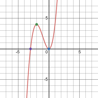
Graph of a degree 3 polynomial

Exercise 3.42 Using the guideline to sketch the curve \(y=\frac{x^2-x}{x^2-3x+2}\).

Solution.

The function is undefined when \(x^2-3x+2=0\) or equivalently, \(x=1\) or \(x=2\). So the domain of the function is \((-\infty, 1)\cup(2, \infty)\).

Note that the function may be simplified \[ y=\frac{x(x-1)}{(x-1)(x-2)}=\frac{x}{x-2}=1+\frac{2}{x-2}. \]

Because \(\lim\limits_{x\to 1}=1+(-2)=-1\). The point \((1, -1)\) is a removable discontinuity.

The function has one \(x\)-intercept \((0, 0)\) which is also the \(y\)-intercept.

Because \[ \lim\limits_{x\to 2^-}\left(1+\frac{2}{x-2}\right)=1+(-\infty)=-\infty \] and \[ \lim\limits_{x\to 2^-}\left(1+\frac{2}{x-2}\right)=1+\infty=\infty \] The function has a vertical asymptote.

Because \[ \lim\limits_{x\to \infty}\left(1+\frac{2}{x-2}\right)=1 \] and \[ \lim\limits_{x\to -\infty}\left(1+\frac{2}{x-2}\right)=1 \] The function has one horizontal asymptote \(y=1\) but no slanted asymptote.

The first derivative is \(y'=-\frac{2}{(x-2)^2}\). So the function has two critical values \(x=1\) and \(x=2\) where the function is undefined.

The second derivative is \(y''=\frac{4}{(x-2)^3}\). The function has no inflection point (Note that the function is undefined at \(x=2\)).

Because the first and second derivative are both continuous over their domains, using test points, we obtain the following table

Interval	Sign of \(y'\)	Sign of \(y''\)	Local Shape of the graph
\((-\infty, 1)\)	\(-\)	\(-\)	decreasing concave downward
\((1, 2)\)	\(-\)	\(-\)	decreasing concave downward
\((2, \infty)\)	\(-\)	\(+\)	decreasing concave upward

Sketching the asymptotes, plotting the intercept, drawing a small empty circle of the removable discontinuity, and then sketching the local graphs, you will see the graph of the curve as shown below.

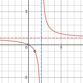
Graph of a rational function with a removable discontinuity

Exercise 3.43 Using the guideline to sketch the curve \(y=(x-1)\sqrt{x+2}\).

Solution.

The function is a real valued function only if \(x+2\ge 0\). So the domain of the function is \([-2, \infty)\).

Solving \((x-1)\sqrt{x+2}=0\) reveals two \(x\)-intercepts \((-2, 0)\) and \((1, 0)\).

When \(x=0\), \(y=-\sqrt2\), so the \(y\)-intercepts is \((0, -\sqrt2)\).

The derivative maybe calculated directly (try it yourself) or in an easier way through a linear substitution \(u=x+2\). After substitution, we get \(y=(u-3)\sqrt{u}=u^{\frac32}-3u^{\frac12}\) and \[ \begin{aligned} \frac{\mathrm{d} y}{\mathrm{d}x}=&\frac{\mathrm{d}y}{\mathrm{d}u}\cdot\frac{\mathrm{d}u}{\mathrm{d}x}\\ =&\frac32u^{\frac12}-\frac32u^{-\frac12}\\ =&\frac32(x+2)^{\frac12}-\frac32(x+2)^{-\frac12} \end{aligned} \] Solving \(\frac{\mathrm{d}y}{\mathrm{d}x}=0\) gives two critical values \(x=-2\) and \(x=-1\).

The second derivative is given by \[ \frac{\mathrm{d}}{\mathrm{d}x}\left(\frac32(x+2)^{\frac12}-\frac32(x+2)^{-\frac12}\right)=\frac{3}{4}(x+2)^{-\frac12}+\frac34x^{-\frac32} \] which is positive over its domain. Therefore, there is no inflection point and the function is concave upward on the interval \((-2, \infty)\).

The function has a vertical asymptote because it’s continuous on the interval \([-2, \infty)\).

Because \[ \lim\limits_{x\to \infty}\left((x-1)\sqrt{x+2}\right)=\infty. \] The function has no horizontal asymptote or slanted asymptote.

Because the first and second derivative are both continuous on their domains, using test points, we obtain the following table

Interval	Sign of \(y'\)	Sign of \(y''\)	Local Shape of the graph
\((-2, -1)\)	\(-\)	\(-\)	decreasing concave upward
\((-1, \infty)\)	\(+\)	\(+\)	increasing concave upward

So at \(x=-1\), the function has local minimum \((-1, -2)\).

Sketching the asymptotes, plotting the intercept, and then sketching the local graphs, you will see the graph of the curve as shown below.

Graph of a function has square root factor

Exercise 3.44 Using the guideline to sketch the curve \(y=\frac{x^2}{x+1}\).

Solution.

The function is undefined if \(x+1=0\). So the domain of the function is \((-\infty, -1)\cup(1, \infty)\).

The function is only one intercept \((0, 0)\).

To find the derivative, again, rewriting the function into a polynomial-like function using substitution will make the calculation easier.

Set \(u=x+1\), then \(x=u-1\). Then \(y=\frac{(u-1)^2}{u}=u-2+u^{-1}=(x+1)-2+(x+1)^{-1}\).

Therefore, the first derivative is \[ y'=1-(x+1)^{-2}=1-\frac{1}{(x+1)^2}. \]

The second derivative is \[ y'=2(x+1)^{-3}=\frac{2}{(x+1)^3}. \]

So the function has two critical values \(x=-2\) and \(x=0\) and one candidate inflection point at \(x=-1\).

Because \(\lim\limits_{x\to -1^-}\frac{x^2}{x+1}=-\infty\) and \(\lim\limits_{x\to -1^+}\frac{x^2}{x+1}=\infty\). The function has a vertical asymptote \(x=-1\).

Because \(y=(x+1)-2+(x+1)^{-1}\), it has a slanted asymptote \(y=(x+1)-2=x-1\).

Because the first and second derivative are both continuous on their domains, using test points, we obtain the following table

Interval	Sign of \(y'\)	Sign of \(y''\)	Local Shape of the graph
\((-\infty, -2)\)	\(+\)	\(-\)	increasing concave downward
\((-2, -1)\)	\(-\)	\(-\)	decreasing concave downward
\((-1, 0)\)	\(-\)	\(+\)	decreasing concave upward
\((0, \infty)\)	\(+\)	\(+\)	increasing concave upward

The function has local maximum \((-2, -4)\) and a local minimum \((0, 0)\).

Sketching the asymptotes, plotting the intercept, and then sketching the local graphs, you will see the graph of the curve as shown below.

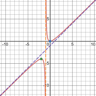
Graph of a function has square root factor

Exercise 3.45 Using the guideline to sketch the curve \(y=\frac{\sin x}{1+\cos x}\).

Solution.

Because \(\sin x\) and \(\cos x\) are periodic with the same period \(2\pi\). So the given function will have the same value when shift \(x\) by \(2\pi\). So we may sketch the graph over one interval of length \(2\pi\) and then using shifting to extend the graph.

Because \(1+\cos x=0\) if \(x=(2k+1)\pi\). We may first restrict the function to the interval \((-\pi, \pi)\) over which the function is well-defined and continuous.

Solve \(\sin x=0\) over the interval \((-\pi,\pi)\), we get \(x=0\). So the function has an \(x\)-intercept \((0, 0)\), which is also the \(y\)-intercept, in the interval \((-\pi, \pi)\).

Because \[ \lim\limits_{x\to -\pi^+}\left(\frac{\sin x}{1+\cos x}\right)=\lim\limits_{x\to -\pi^+}\left(\frac{2\sin \frac x2\cos\frac x2}{2\cos^2\frac x2}\right)=-\infty \] and \[ \lim\limits_{x\to \pi^-}\left(\frac{\sin x}{1+\cos x}\right)=\lim\limits_{x\to \pi^-}\left(\frac{2\sin \frac x2\cos\frac x2}{2\cos^2\frac x2}\right)=\infty \]

The function has vertical asymptotes at where it is undefined, i.e. \(x=(2k+1)\pi\).

The function has one horizontal asymptote because it is periodic.

To find the first derivative and second derivative, you may rewrite the function as \(y=\tan\frac x2\) first or apply the quotient rule directly. Here, I will show the quotient rule method.

The first derivative is \[ y'=\frac{\cos x(1+\cos x)-\sin x(-\sin x)}{(1+\cos x)^2}=\frac{1}{1+\cos x}. \]

So \(y'>0\) on the interval \((-\pi, \pi)\).

The second derivative is \[ y''=\left(\frac{1}{1+\cos x}\right)'=-\frac{2\sin x}{(1+\cos x)^2}. \]

So the function has an candidate inflection point at \(x=0\).

Because the first and second derivative are both continuous over the interval \((-\pi, \pi)\), using test points, we obtain the following table

Interval	Sign of \(y'\)	Sign of \(y''\)	Local Shape of the graph
\((-\pi, 0)\)	\(+\)	\(-\)	increasing concave downward
\((0, \pi)\)	\(+\)	\(+\)	increasing concave upward

Sketching the asymptotes, plotting the intercept, sketching the local graphs, and then shifting the graph to other periods, you will see the graph of the curve as shown below.

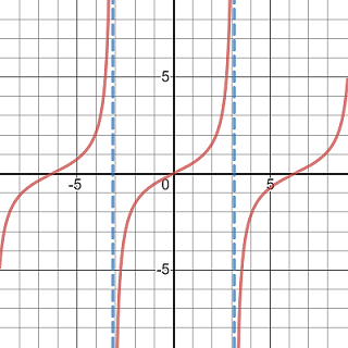
Graph of the function defined as tangent of half angle

3.6 Optimization Problems

The key to solve an optimization problem is to translate the problem into a function (defined by an equation). To be more precise, the following problem strategy may be applied.

1. Understand the Problem and represent known and unknown quantities using variables and expressions. In this step, it is useful to draw a diagram and identify variables and expressions on the diagram.
2. Write any equations relating the variables.
3. Determine which quantity is to be maximized or minimized. Find the range of values of the other variables if possible.
4. Express the quantity to be maximized or minimized as an explicitly define function of other variables.
5. Locate the maximum or minimum value of the function.

Exercise 3.46 Find the dimension of the rectangle with the largest area among all rectangles that have a perimeter 100 cm.

Solution.

Suppose the length of the rectangle is \(x\). Then the width of the rectangle is \(\frac{100-2x}{2}=50-x\) because the perimeter is 100.

The area of the rectangle is a function of the length \[ A(x)=x(50-x)=50x-x^2, \qquad 0<x<50. \]

To find the largest possible area, we may use the first derivative test. Because \(A'(x)=50-2x\). So \(A(x)\) has a local extreme value at \(x=25\). Because \(A'(x)>0\) for \(x<25\) and \(A'(x)>0\) for \(x>25\). Then \(A(25)=25^2=625 ~\text{cm}^2\) is the largest area among all rectangles with the perimeter 100 cm.

The dimension of that rectangle is 25 cm by 25 cm.

Exercise 3.47 An open-top rectangular box is to be made from a rectangular shaped cardboard measured 12 inches by 18 inches by removing a square from each corner of the box and folding up the flaps on each side. What size square should be cut out of each corner to get a box with the maximum volume?

Solution.

Suppose the length of a side of a square corner to be removed is \(x\) inches.

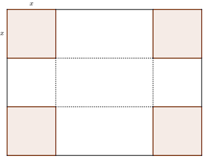
Picture of a cardboard with four square conners highlighted

Note that \(x\), \(18-2x\) and \(12-2x\) should be all positive number.

So the volume \(V\) of the box is a function of \(x\) \[ V(x)=x(18-2x)(12-2x)=4(x^3-15x^2+54x), \qquad 0<x<6. \]

The first derivative is \[ V'(x)=4(3x^2-30x+54)=12(x^2-10x+18). \] It has one critical value \(x=5-\sqrt{7}\) in the interval \((0, 6)\).

Because \(V'(x)>0\) when \(0<x<5-\sqrt7\) and \(V'(x)>0\) when \(5-\sqrt7<x<6\). The largest possible volume of the box is \(V(5-\sqrt7)\).

The box to be cut out should have a side length \(5-\sqrt7\) inches so that the box has the largest volume.

Exercise 3.48 A cylindrical can is to be made to hold 1 L of tomato sauce. Find the dimensions that will minimize the cost of the metal to manufacture the can.

Solution.

Suppose the radius of the bottom disk is \(r\). The the height of the can is \(h=\frac{1}{\pi r^2}\).

To create such a can, we need two metal disks with radius \(r\) for the top and bottom and the rectangle piece with dimension \(h\) by \(2\pi r\) for the side of the can.

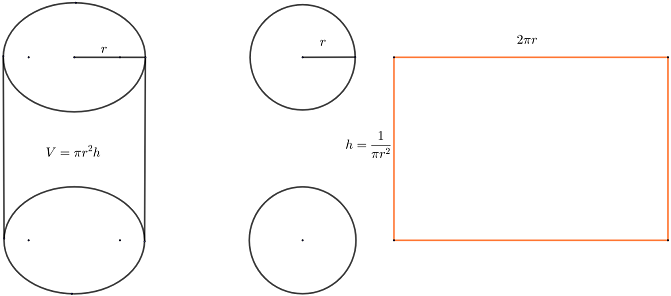
A picture of cylindrical can

The area can be expressed as a function of \(r\) \[ A(r)=2\pi r^2+2\pi rh=2\pi r^2+\frac{2}{r}, \quad 0< r<\infty \] Then \[ A'(r)=4\pi r-\frac{2}{r^2}. \]

The function \(A(r)\) has one critical value \(r=\frac{\sqrt[3]{4\pi^2}}{2\pi}\) in its domain.

To minimize the cost, the base of the can should be \(\frac{\sqrt[3]{4\pi^2}}{2\pi}\), the height should be \(\frac{\sqrt[3]{4\pi^2}}{\pi}\).

Exercise 3.49 A boat leaves a dock at 12:00 pm and travels due south at a speed of 20 m/h. Another boat has been heading due east at 15 m/h and reaches the same dock at 1:00 pm. At what time were the two boats closest together?

Solution.

Let’s call the boat heading south \(A\) and the other one \(B\). Denote the docker by \(D\).

After \(t\) hours (\(0\le t\le 1\)), the boat \(A\) is \(20t\) m away from the dock. The boat \(B\) is \(15-15t\) away from the dock.

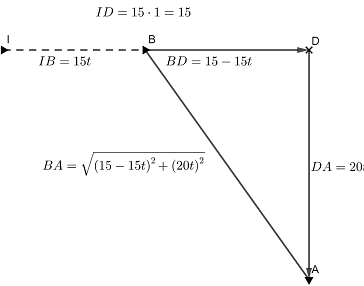
A picture shows positions of two boat away from a dock

The distance between the boats is a function of the time \(t\) \[ d(t)=\sqrt{(15-15t)^2+(20t)^2}=5\sqrt{25t^2-18t+9} \] with \(0\le t\le 1\).

The derivative function is \[ d'(t)=\frac{5(25t-9)}{\sqrt{25t^2-18t+9}}. \]

There is a critical value \(t=\frac{9}{25}\).

Because \(d'(t)<0\) when \(t<\frac{9}{25}\) and \(d'(t)>0\) when \(t>\frac{9}{25}\).

The distance reaches its minimum when \(t=\frac{9}{25}\).

Exercise 3.50 A tennis ball player plays in a stadium that holds 4500 spectators. With ticket prices at $ 15, the average attendance had been 2500. When ticket prices were lowered to $10, the average attendance rose to 3500.

1. Find the demand function, assuming that it is linear.
2. How should ticket prices be set to maximize revenue?

Solution.

Suppose the price is $ \(x\). Because the demand function \(D(x)\) is linear and we know that \(D(15)=2500\) and \(D(10)=3500\). So the demand function has the slope \(m=-200\). The demand function can be written as \[ D(x)=-200(x-10)+3500=-200x+3700, \quad x>0. \]

The revenue is given by \[ R(x)=xD(x)=x(3700-200x). \]

The first derivative function is \[ R'(x)=3700-400x. \]

Because \(R'(t)>0\) when \(t<\frac{37}{4}\) and \(R'(t)<0\) when \(x>\frac{37}{4}\).

So when the price is $9.25, the revenue reaches its maximum.

3.7 Antiderivatives

A function \(F\) is called an antiderivative of a function \(f\) on an interval \(I\) if \(F'(x)=f(x)\) for all \(x\in I\).

By the mean value theorem, if \(F\) is an antiderivative of \(f\) on an interval \(I\). then the most general antiderivative of \(f\) on \(I\) is \(F(x)+C\), where \(C\) is an arbitrary constant.

By rule of derivatives, we have the following table of antiderivatives.

Function	An antiderivative
\(af+bg\)	\(aF+bG\)
\(x^n\), \(n\neq -1\)	\(\frac{x^{n+1}}{n+1}\)
\(\sin x\)	\(-\cos x\)
\(\cos x\)	\(\sin x\)
\(\sec^2x\)	\(\tan x\)
\(\sec x\tan x\)	\(\sec x\)

In the above table, \(F\) and \(G\) are antiderivative of \(f\) and \(g\) respectively, \(a\) and \(b\) are arbitrary constants.

Exercise 3.51 Find the most general antiderivative of the function \(f(x)=3x^2-2x+1\).

Solution.

The general antiderivative is \[ \begin{aligned} F(x)=&3\cdot\frac{x^{2+1}}{2+1}-2\cdot\frac{x^{1+1}}{1+1}+x+C\\ =&x^3-x^2+x+C. \end{aligned} \]

Exercise 3.52 Find the most general antiderivative of the function \(f(x)=\sqrt{x}-x^5\).

Solution.

The general antiderivative is \[ \begin{aligned} F(x)=&\frac{x^{\frac12+1}}{\frac12+1}-\frac{x^{5+1}}{5+1}+C\\ =&\frac{2x^{\frac32}}{3}-\frac{x^6}{6}+C. \end{aligned} \]

Exercise 3.53 Find the most general antiderivative of the function \(f(x)=x^{-\frac12}-x^{\frac13}\).

Solution.

The general antiderivative is \[ \begin{aligned} F(x)=&\frac{x^{-\frac12+1}}{-\frac12+1}-\frac{x^{\frac13+1}}{\frac13+1}+C\\ =&2x^{\frac12}-\frac34x^{\frac43}+C. \end{aligned} \]

Exercise 3.54 Find the most general antiderivative of the function \(f(x)=\frac{x-3x^2+2}{\sqrt{x}}\).

Solution.

First rewrite the function as a polynomial-liked function \[ \begin{aligned} f(x)=&\frac{x-3x^2+2}{\sqrt{x}}\\ =&\frac{x-3x^2+1}{x^{\frac12}}\\ =&x^{\frac12}-3x^{\frac32}+x^{-\frac12} \end{aligned} \]

Then the general antiderivative is \[ \begin{aligned} F(x)=&\frac{x^{\frac12+1}}{\frac12+1}-3\frac{x^{\frac32+1}}{\frac32+1}+\frac{x^{-\frac12+1}}{-\frac12+1}+C\\ =&\frac{2x^{\frac32}}{3}-\frac{6x^{\frac52}}{5}+2x^{\frac12}+C. \end{aligned} \]

Exercise 3.55 Find the most general antiderivative of the function \(f(x)=3\sec^2x-\sin x-\frac{1}{x^2}\).

Solution.

The general antiderivative is \[ \begin{aligned} F(x)=&3\tan x-(-\cos x)-\frac{x^{-2+1}}{-2+1}+C\\ =&3\tan x+\cos x+\frac1x+C. \end{aligned} \]

Exercise 3.56 Find the antiderivative \(F\) of the function \(f(x)=3x-2x^3\) such that \(F(1)=0\).

Solution.

First we find the general antiderivative: \[ \begin{aligned} F(x)=&3\frac{x^{1+1}}{1+1}-2\frac{x^{3+1}}{3+1}+C\\ =&\frac{3x^{2}}{2}-\frac{x^{4}}{2}+C. \end{aligned} \]

Because \(F(1)=\frac{3}{2}-\frac{1}{2}+C=0\). Then \(C=-1\) and the function \(F\) is given by \[ F(x)=\frac{3x^{2}}{2}-\frac{x^{4}}{2}-1. \]

Exercise 3.57 Find the function \(f\) such that \(f''(x)=3\cos x-2\sin x+\frac{4}{3\sqrt[3]{x}}\).

Solution.

The first derivative is \[ \begin{aligned} f'(x)=&3\sin x-2(-\cos x)+\frac{4}{3}\frac{x^{-\frac13+1}}{-\frac13+1}+C_1\\ =&3\sin x+2\cos x+2x^{\frac23}+C_1. \end{aligned} \]

The function \(f\) is then given by \[ \begin{aligned} f'(x)=&3(-\cos x)+2\sin x+2\frac{x^{\frac23+1}}{\frac23+1}+C_1x+C_2\\ =&-3\cos x+2\sin x+\frac{6x^{\frac53}}{5}+C_1x+C_2. \end{aligned} \]

Exercise 3.58 Find the function \(f\) such that \(f'''(x)=\cos x\), \(f(0)=3\), \(f'(0)=2\), and \(f''(0)=1\).

Solution.

The most general second derivative is \[ f''(x)=\sin x+C_1. \] Because \(f''(0)=\sin 0+C_1 = 1.\) Then \(C_1=1\) and \(f''(x)=\sin x+1\).

The most general first derivative is \[ f'(x)=-\cos x+x+C_2. \] Because \(f'(0)=-\cos 0+0+C_2 = 2.\) Then \(C_2=3\) and \(f'(x)=-\cos x+x+3\).

The general form of the function is \[ f(x)=-\sin x+\frac{x^2}{2}+3x+C_3. \] Because \(f(0)=-\sin 0+0+0+C_3 = 3.\) Then \(C_3=3\) and \(f(x)=-\sin x+\frac{x^2}{2}+3x+3\).

Exercise 3.59 Find a function \(f\) such that \(f'(x)=x^3\) and the line \(x-y=0\) is tangent to the graph of \(f\).

Solution.

The slope of the tangent line is \(m=1\). Solve \(f'(x)=x^3=1\), we get the \(x\)-coordinate of the tangent point \(x=1\). The tangent point is then \((1, f(1))=(1, 1)\) because the tangent point is also on the tangent line \(x-y=0\).

The most general antiderivative of \(f'\) is \[ f(x)=\frac{x^4}{4}+C. \]

Because \(f(1)=\frac14+C=1\). The function \(f\) is given by \[ f(x)=\frac{x^4}{4}+\frac34. \]

Exercise 3.60 A particle is moving with a initial velocity \(v(0)=-2\). The acceleration is given by \(a(t)=-2t+1\) with \(s(0)=5\). Find the position of the particle.

Solution.

The velocity is an antiderivative of the acceleration function. Therefore, \(v\) has the form \[ v(t)=-t^2+t+C_1. \]

Because \(v(0)=C_1=-2\). Then \(v(t)=-t^2+t-2\).

The position function is an antiderivative of the velocity function. It has a general form \[ s(t)=-\frac{t^3}{3}+\frac{t^2}{2}-2t+C_2. \]

Because \(s(0)=C_2=5\). Then the position function is given by \[ s(t)=-\frac{t^3}{3}+\frac{t^2}{2}-2t+5. \]