\newcommand{\ii}{\mathbf{i}} \newcommand{\parll}{ {\mathbin{\parallel}} } \newcommand{\prll}{{\mathbin{\!/\mkern-5mu/\!}}}

Topic 2 Derivatives

2.1 Derivatives as Rate of Changes

A derivative of a function is a special type of limit in the sense that it represents the instantaneous rate of change.

Definition 2.1 Given a function f defined near a, the average rate of change (or difference quotient) near a is \frac{f(x)-f(a)}{x-a}. The derivative of a function f at a number a, denoted by f'(a) (read as f prime of a) is defined as f'(a)=\lim\limits_{x\to a}\frac{f(x)-f(a)}{x-a} if this limit exists.
We say that f is differentiable at a if the limit \lim\limits_{x\to a}\frac{f(x)-f(a)}{x-a} exists.

By a substitution x=a+h, we see that f'(a)=\lim\limits_{h\to 0}\frac{f(a+h)-f(a)}{h}.

The slope of a tangent line and an instantaneous velocity are both derivatives.

In terms of the derivative, an equation of the tangent line through (a, f(a)) can be written as y=f'(a)(x-a)+f(a). The equation is known as the point-slope form equation.

Exercise 2.1 Find the tangent line to the curve defined by y=\sqrt{x} at the point (1, 1).

Solution.

The slope of the tangent line is given by the limit \begin{aligned} \lim_{x\to 1}\frac{f(x)-f(1)}{x-1}&=\lim_{x\to 1}\frac{\sqrt{x}-1}{x-1}\\ &=\lim_{x\to1}\frac{1}{\sqrt{x}+1}\\ &=\frac{1}{2}. \end{aligned} An equation of tangent line is y=\frac12(x-1)+1.

Exercise 2.2 Find the derivative f'(2) for the function f(x)=3x^2-2x+1.

Solution.

The derivative (if exists) is the limit of difference quotient \begin{aligned} f'(2)=&\lim_{x\to 2}\frac{f(x)-f(2)}{x-2}\\ =&\lim_{x\to 2}\frac{(3x^2-2x+1)-(3\cdot 2^2-2\cdot 2+1)}{x-2}\\ =&\lim_{x\to 2}\frac{(3x+4)(x-2)}{x-2}\\ =&\lim_{x\to 2}(3x+4)=10. \end{aligned}

Exercise 2.3 An equation of the tangent line to the curve y=f(x) at the point where x=2 is y=x-2. Find f(2) and f'(2).

Solution.

The derivative of the function at x=a is the same as the slope of the tangent line through (a, f(a)). Since the slope of the tangent line when x=2 is 1, we know that f'(2)=1. As the function and the tangent line touch each other at x=2, we see that f(2)=2-2=0.

Exercise 2.4 Find f'(a) for the function f(x)=\frac1{x-1}, where a is a number and a\neq 1.

Solution.

By the definition of derivative, we have \begin{aligned} f'(a)&=\lim_{x\to a}\dfrac{f(x)-f(a)}{x-a}\\ &=\lim_{x\to a}\dfrac{\frac{1}{x-1}-\frac{1}{a-1}}{x-a}\\ &=\lim_{x\to a}\dfrac{\frac{a-x}{(x-1)(a-1)}}{x-a}\\ &=\lim_{x\to a}\dfrac{-1}{(x-1)(a-1)}\\ &=-\dfrac{1}{(a-1)^2} \end{aligned}

Exercise 2.5 The limit \lim\limits_{h\to 0}\frac{\frac{2}{\sqrt{4+h}}-1}{h} represents the derivative of some function f at some number a. State f and a.

Solution.

The derivative of a function f can be calculated using f'(a)=\lim\limits_{h\to 0}\frac{f(a+h)-f(a)}{h}.

Comparing with the limit given in the question, we may assume that a=2 and f(x)=\frac{2}{\sqrt{x}}. It can be checked that f(2+h)=\frac{2}{\sqrt{4+h}} and f(2)=1.

2.2 Derivative as a Function

Definition 2.2 If f is differentiable at every point in an interval I, the we say f is differentiable over I.

For a function f differentiable over an interval I, we may obtain a new function by a unique value f'(x) to each x in I. We call the function y=f'(x) the derivative function (or simply derivative) of f.

Using the identity f(x)-f(a)=(x-a)\cdot\frac{f(x)-f(a)}{x-a} and limit laws, we obtain easily the following theorem.

Theorem 2.1 If the function f is differentiable at a, then f is continuous at a.

When a function is given in the form y=f(x), we also use y' to denote the derivative function. The notations f' and y' are known as Lagrange’s “prime” notation.

As the derivative function is essentially (the limit) a difference quotient, we also use \frac{\mathrm{d}y}{\mathrm{d x}} (or \mathrm{d}y/\mathrm{d x}) to denote the derivative functions. The notation \frac{\mathrm{d}y}{\mathrm{d x}} was introduced by Leibniz and called Leibniz’s notation.

A worthful remark is that \mathrm{d}x and \mathrm{d} y may be considered as variables and are called differentials.

The process of calculating a derivative is known as differentiation. We view the prime ' or better the notation \frac{\mathrm{d}}{\mathrm{d}x} as an operator and call it the differential operator.

Sometimes, a differential operator is also denoted as D or D_x to indicate the independent variable x. Those notations are known as Euler’s notation.

Higher derivatives are defined as repeated differentiations of functions. The second derivative f''(x)=(f'(x))' is the derivative of the first derivative of f. The third derivative is f'''(x)=(f''(x))'. The n-th derivative is defined recursively as f^{(n)}(x)=(f^{(n-1)}(x))'.

Exercise 2.6 Use the definition of derivative to find f'(x) for f(x)=1-2x.

Solution.

By the definition of derivative, we have \begin{aligned} f'(x)&=\lim_{h\to 0}\dfrac{f(x+h)-f(x)}{h}\\ &=\lim_{h\to 0}\dfrac{(1-2(x+h))-(1-2x)}{h}\\ &=\lim_{h\to 0}\dfrac{-2h}{h}\\ &=-2. \end{aligned}

Exercise 2.7 Use the definition of derivative to find f'(x) for f(x)=x^3-x^2.

Solution.

By the definition of derivative, we have \begin{aligned} f'(x)&=\lim_{h\to 0}\dfrac{f(x+h)-f(x)}{h}\\ &=\lim_{h\to 0}\dfrac{((x+h)^3-(x+h)^2)-(x^3-x^2)}{h}\\ &=\lim_{h\to 0}\dfrac{((x+h)^3-x^3)-((x+h)^2-x^2)}{h}\\ &=\lim_{h\to 0}((x+h)^2+x(x+h)+x^2-(2x+h))\\ &=3x^2-2x \end{aligned}

Exercise 2.8 Use the definition of derivative to find f'(x) for f(x)=\frac{1}{x-2}.

Solution.

By the definition of derivative, we have \begin{aligned} f'(x)&=\lim_{h\to 0}\dfrac{f(x+h)-f(x)}{h}\\ &=\lim_{h\to 0}\dfrac{\frac{1}{x+h-2}-\frac{1}{x-2}}{h}\\ &=\lim_{h\to 0}\dfrac{-h}{h(x+h-2)(x-2)}\\ &=-\dfrac{1}{(x-2)^2} \end{aligned}

Exercise 2.9 Use the definition of derivative to find f'(x) for f(x)=\frac{1}{\sqrt{x+1}}.

Solution.

By the definition of derivative, we have \begin{aligned} f'(x)&=\lim_{h\to 0}\dfrac{f(x+h)-f(x)}{h}\\ &=\lim_{h\to 0}\dfrac{\frac{1}{\sqrt{x+h+1}}-\frac{1}{\sqrt{x+1}}}{h}\\ &=\lim_{h\to 0}\dfrac{\sqrt{x+1}-\sqrt{x+h+1}}{h\sqrt{x+h+1}\sqrt{x+1}}\\ &=\lim_{h\to 0}\dfrac{1}{\sqrt{x+h+1}\sqrt{x+1}}\lim_{h\to 0}\dfrac{\sqrt{x+1}-\sqrt{x+h+1}}{h}\\ &=\dfrac{1}{x+1}\cdot \frac{-1}{2\sqrt{x+1}}\\ &=-\frac{1}{2(x+1)\sqrt{x+1}} \end{aligned}

Exercise 2.10 Use the definition of derivative to find f'(x) for f(x)=x+\frac1x.

Solution.

By the definition of derivative, we have \begin{aligned} f'(x)&=\lim_{h\to 0}\dfrac{f(x+h)-f(x)}{h}\\ &=\lim_{h\to 0}\dfrac{((x+h)+\frac1{x+h})-(x+\frac1x)}{h}\\ &=\lim_{h\to 0}\dfrac{h+\frac{-h}{x(x+h)}}{h}\\ &=\lim_{h\to 0}\left(1-\frac{1}{x(x+h)}\right)\\ &=1-\frac{1}{x^2} \end{aligned}

Exercise 2.11 Sketch the derivative function of the following function.

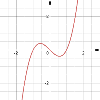
The graph of a x^3-x

Solution.

The derivative function is a parabola.

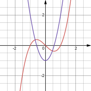
The graphs of x^3-x and its derivative

Exercise 2.12 Find the value a where the function f(x)=|x-5| is not differentiable

Solution.

When x<5 or x>5, the function is a linear function and hence differentiable. It may not be differentiable at x=5. We can check that using the definition of differentiability. Calculate one-side limits because the absolute value sign is involved. \lim_{x\to 5^-}\frac{f(x)-f(5)}{x-5}=\lim_{x\to 5^-}\frac{|x-5|-0}{x-5}\lim_{x\to 5^-}\frac{5-x}{x-5}=-1. \lim_{x\to 5^+}\frac{f(x)-f(5)}{x-5}=\lim_{x\to 5^+}\frac{|x-5|-0}{x-5}\lim_{x\to 5^+}\frac{x-5}{x-5}=1. Because the left and right limits do not agree, the limit of the difference quotient does not exist and the function is not differentiable at x=5.

Exercise 2.13 Find the values of x where the function f given in the following graph is not differentiable. Explain why f is not differentiable at the values you found.

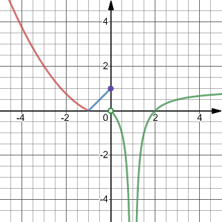
A function whose derivative function has three types of discontinuity

Solution.

If f is differentiable at x=a, then it is continuous at x=a and it can be approximated by the tangent line locally, that is, the graph is locally flat.

In the graph, we see that f is not continuous at x=0 and not defined at x=1. So f cannot be differentiable at those two values. Besides, when x=-1, the graph is not flat. So f is not differentiable at x=-1 too.

We can conclude that f has three discontinuities x=-1, x=0 and x=1.

Exercise 2.14 Find values of a and b in the function f(x)= \begin{cases} ax+b & x>=1\\ x^2-3 & x<1 \end{cases} such f is differentiable.

Solution.

To make f is differential, it must be continuous at x=1 and the left derivative and right derivative much agree. Those conditions produces the following system of equations \begin{cases} a+b=1-3\\ a=2 \end{cases}

Solve for b, we get b=-4.

Note that the second equation is from the one side limits of the difference quotients.

Exercise 2.15 Use the definition of derivative to find f'(x) and f''(x) for f(x)=3x^2-2x-1.

Solution.

By the definition of derivative, we have \begin{aligned} f'(x)&=\lim_{h\to 0}\dfrac{f(x+h)-f(x)}{h}\\ &=\lim_{h\to 0}\dfrac{(3(x+h)^2-2(x+h)-1)-(3x^2-2x-1)}{h}\\ &=\lim_{h\to 0}\dfrac{6xh-3h^2-2h}{h}\\ &=\lim_{h\to 0}\left(6x-2-3h\right)\\ &=6x-2 \end{aligned} \begin{aligned} f''(x)&=\lim_{h\to 0}\dfrac{f'(x+h)-f'(x)}{h}\\ &=\lim_{h\to 0}\dfrac{(6(x+h)-2)-(6x-2)}{h}\\ &=\lim_{h\to 0}\dfrac{6h}{h}\\ &=6 \end{aligned}

2.3 Differentiation Formulas

Using limit laws, you may obtain the following differential formulas.

Theorem 2.2   1. Constant rule: Let c be a constant number. If f(x)=c, then f'(x)=0. 2. Power rule: Let n be a real number. If f(x)=x^n, then f'(x)=nx^{n-1}.

Theorem 2.3 Let f and g be differentiable functions and c be a constant number.

1. Scalar multiplication rule: Let c be a constant number. Then (cf)'=cf'(x).
2. Sum rule: (f+g)'=f'+g'.
3. Product rule: (fg)'=f'g+fg'.
4. Quotient rule: \left(\dfrac{f}{g}\right)'=\dfrac{f'g-fg'}{g^2}.

Exercise 2.16 Find f'(x) for f(x)=x^{2019}+9.

Solution.

f'(x)=(x^{2019}+9)'=(x^{2019})'+(9)'=2019x^{2018}.

Exercise 2.17 Find f'(x) for f(x)=x^{3}-\frac{1}{x^2}.

Solution.

f'(x)=\left(x^{3}-\frac{1}{x^2}\right)'=(x^3)'-(x^{-2})'=3x^2+2x^{-3}.

Exercise 2.18 Find f'(x) for f(x)=(x+3)(3x^2-1).

Solution.

First simplify the function rule. f(x)=(x+3)(3x^2-1)=3x^3+9x^2-x-3

Now it should be easier to calculate the derivative. f'(x)=\left(3x^3+9x^2-x-3\right)'=9x^2+18x-1.

Exercise 2.19 Find \frac{\mathrm{d} y}{\mathrm{d} x} for y=\frac{2}{3x^{2/3}}.

Solution.

Rewrite using negative exponents. y=\frac{2}{3x^{2/3}}=\frac23x^{-\frac23} The derivative is \frac{\mathrm{d} y}{\mathrm{d} x}=\frac{\mathrm{d}}{\mathrm{d} x}\left(\frac23x^{-\frac23}\right)=-\frac49x^{-\frac53}.

Exercise 2.20 Find \frac{\mathrm{d} y}{\mathrm{d} x} for y=x(2\sqrt{x}-1).

Solution.

Rewrite using exponents first. y=x(2\sqrt{x}-1)=2x^{\frac32}-x The derivative is \frac{\mathrm{d} y}{\mathrm{d} x}=\frac{\mathrm{d}}{\mathrm{d} x}\left(2x^{\frac32}-x\right)=3x^\frac12-1=3\sqrt{x}-1.

Exercise 2.21 Find A'(R) for A(R)=\pi R^2.

Solution.

The derivative is A'(R)=(\pi R\cdot R)'=\pi((R)'R+R(R'))=2\pi R.

Exercise 2.22 Find g'(x) for g(x)=\frac{3x^2+5x-7}{\sqrt{x}}.

Solution.

Rewrite using exponents first. g(x)=\frac{3x^2+5x-7}{\sqrt{x}}=3x^{\frac32}+5x^{\frac12}-7x^{-\frac12} The derivative is \begin{aligned} g'(x)=&\left(3x^{\frac32}+5x^{\frac12}-7x^{-\frac12}\right)'\\ =&\frac92x^{\frac12}+\frac52x^{-\frac12}+\frac72x^{-\frac32}\\ =&\dfrac{9x^2+5x+7}{2x\sqrt{x}} \end{aligned}

Exercise 2.23 Find h'(t) for h(t)=\frac{t^3-1}{t^2+1}.

Solution.

Apply the quotient rule. \begin{aligned} h'(t)=&\left(\dfrac{t^3-1}{t^2+1}\right)'\\ =&\dfrac{(t^3-1)'(t^2+1)-(t^3-1)(t^2+1)'}{(t^2+1)^2}\\ =&\dfrac{3t^2(t^2+1)-2t(t^3-1)}{(t^2+1)^2}\\ =&\dfrac{t^4+3t^2+2t}{(t^2+1)^2}\\ \end{aligned}

Exercise 2.24 Find \frac{\mathrm{d} s}{\mathrm{d} t} for s=\left(\frac{1}{t}-\frac{1}{\sqrt{t}}\right)^{2}.

Solution.

Simplify and rewrite using exponents first. s=\left(\frac{1}{t}-\frac{1}{\sqrt{t}}\right)^{2}=t^{-2}-2t^{-\frac32}+t^{-1} The derivative is \begin{aligned} \frac{\mathrm{d} s}{\mathrm{d} t}=&\frac{\mathrm{d}}{\mathrm{d} t}\left(t^{-2}-2t^{-\frac32}+t^{-1}\right)\\ =&-2t^{-3}+3t^{-\frac52}-t^{-2} \end{aligned}

Exercise 2.25 Find f'(x) for f(x)=\frac{x(x+2)^{2}}{1-x}.

Solution.

Apply the quotient rule. \begin{aligned} f'(x)=&\left(\frac{x(x+2)^{2}}{1-x}\right)'\\ =&\dfrac{(x(x+2)^{2})'(1-x)-(x(x+2)^{2})(1-x)'}{(x-1)^2}\\ =&\dfrac{(3x^2+8x+4)(1-x)+(x^3+4x^2+4x)}{(x-1)^2}\\ =&\dfrac{-2x^3-x^2+8x+4}{(x-1)^2}\\ \end{aligned}

Exercise 2.26 Find f'(x) for f(x)=(x^3-3x^2+3x-1)(x^2+2).

Solution.

Apply the product rule. \begin{aligned} f'(x)=&\left((x^3-3x^2+3x-1)(x^2+2)\right)'\\ =&(x^3-3x^2+3x-1)'(x^2+2)+(x^3-3x^2+3x-1)(x^2+2)'\\ =&(3x^2-6x+3)(x^2+2)+2x(x^3-3x^2+3x-1)\\ =&5x^4-12x^3+15x-14x+6\\ \end{aligned}

Note that you may also simplify the function first.

Exercise 2.27 Find f'(x) for f(x)=\frac{\sqrt[3]{x}}{x-1}.

Solution.

Apply the quotient rule. \begin{aligned} f'(x)=&\left(\dfrac{\sqrt[3]{x}}{x-1}\right)'\\ =&\dfrac{(x^{\frac13})'(x-1)-x^{\frac13}(x-1)'}{(x-1)^2}\\ =&\dfrac{\frac13x^{-\frac23}(x-1)-x^{\frac13}}{(x-1)^2}\\ =&\dfrac{-2x-1}{3\sqrt[3]{x^2}(x-1)^2} \end{aligned}

Exercise 2.28 Suppose that f and g are both differentiable functions with f(4)=3, g(4)=2, f'(4)=9 and g'(4)=5. Find h'(4) where h(x)=\frac{2}{\sqrt{x}}-\frac{f(x)-1}{g(x)}.

Solution.

By rules of derivatives, \begin{aligned} h'(x)=&\left(\frac{2}{\sqrt{x}}-\frac{f(x)-1}{g(x)}\right)'\\ =&(2x^{-\frac12})'-\frac{(f(x)-1)'g(x)-(f(x)-1)g'(x)}{(g(x))^2}\\ =&-x^{-\frac32}-\frac{f'(x)g(x)-(f(x)-1)g'(x)}{(g(x))^2}\\ \end{aligned}

Therefore, h'(4)=-4^{-\frac32}-\frac{f'(4)g(4)-(f(4)-1)g'(4)}{(g(4))^2}=-\frac{17}{8}.

Exercise 2.29 Find equations of the tangent line and normal line to the curve y=4\sqrt{x}-x at (1,3).

Solution.

The derivative of the function is \frac{\mathrm{d} y}{\mathrm{d} x}=\frac{2}{\sqrt{x}}-1. The slope of the tangent line is the value of the derivative function at x=1, that is, m=\frac{\mathrm{d} y}{\mathrm{d} x}\bigg|_{x=1}=\frac2{\sqrt{1}}-1=1 So the tangent line is y=x+1.

The normal line is the line that is perpendicular to the tangent line and passing through the tangent point. The slope of the normal line passing through (a, f(a)) (if it is not vertical) is -\frac{1}{f'(a)}.

In this question, the slope of the normal line is -1. Then an equation of the normal line is y=-x+4.

Exercise 2.30 Find the second derivatives of the function f(x)=\frac{x}{1-x}.

Solution.

You may apply the quotient rule directly. Here, we rewrite the function first. f(x)=\frac{x}{1-x}=-1+\frac{1}{1-x} Then \begin{aligned} f'(x)=&\left(-1+\frac{1}{1-x}\right)'\\ =&\left(\frac{1}{1-x}\right)'\\ =&\frac{-(1-x)'}{(1-x)^2}\\ =&\frac{1}{(1-x)^2}\\ \end{aligned} The second derivative is \begin{aligned} f'(x)=&\left(\frac{1}{(1-x)^2}\right)'\\ =&\frac{-((1-x)^2)'}{(1-x)^4}\\ =&\frac{-(1-2x+x^2)'}{(1-x)^4}\\ =&\frac{2-2x}{(1-x)^4}\\ =&\frac{2}{(1-x)^3}. \end{aligned}

2.4 Derivatives of Trigonometric Functions

Using trigonometric identities, the limit \lim\limits_{h\to 0}\frac{\sin h}{h}=1 and derivative rules, you may find derivatives of trigonometric functions as shown below. \begin{aligned} \dfrac{\mathrm{d}}{\mathrm{d} x}\sin x &= \cos x \\ \dfrac{\mathrm{d}}{\mathrm{d} x}\cos x &= -\sin x\\ \dfrac{\mathrm{d}}{\mathrm{d} x}\tan x &= \sec^2x\\ \end{aligned} \qquad \begin{aligned} \dfrac{\mathrm{d}}{\mathrm{d} x}\csc x &= -\csc x \cot x \\ \dfrac{\mathrm{d}}{\mathrm{d} x}\sec x &= \sec x\tan x\\ \dfrac{\mathrm{d}}{\mathrm{d} x}\cot x &= -\csc^2x\\ \end{aligned}

Exercise 2.31 Find the derivatives of the function f(x)=2x^2\cos x.

Solution.

\begin{aligned} f'(x)=&\left(2x^2\cos x\right)'\\ =&2((x^2)'\cos x+x^2(\cos x)')\\ =&2(2x\cos x-x^2\sin x)\\ =&4x\cos x-x^2\sin x. \end{aligned}

Exercise 2.32 Find the derivatives of the function f(x)=\sin x \cos x.

Solution.

\begin{aligned} f'(x)=&\left(\sin x\cos x\right)'\\ =&(\sin x)'\cos x+\sin x(\cos x)'\\ =&\cos^2x-\sin^2x=\cos(2x). \end{aligned}

Exercise 2.33 Find the derivatives of the function f(x)=\frac{\sin x}{x+1}.

Solution.

\begin{aligned} f'(x)=&\left(\frac{\sin x}{x+1}\right)'\\ =&\frac{(\sin x)'(x+1)-\sin x(x+1)'}{(x+1)^2}\\ =&\frac{(x+1)\cos x-\sin x}{(x+1)^2}. \end{aligned}

Exercise 2.34 Find the derivatives of the function f(x)=2\tan x+\sqrt{x^3}.

Solution.

\begin{aligned} f'(x)=&\left(2\tan x+\sqrt{x^3}\right)'\\ =&2(\tan x)'+(x^{\frac23})'\\ =&2\sec^2x+\frac32x^{\frac12}. \end{aligned}

Exercise 2.35 Find the derivatives of the function f(x)=2\tan x-x\sec x.

Solution.

\begin{aligned} f'(x)=&\left(2\tan x-x\sec x\right)'\\ =&2(\tan x)'+(x\sec x)'\\ =&2\sec^2x+\sec x+x(\sec x)'\\ =&2\sec^2x+\sec x+x\tan x\sec x. \end{aligned}

Exercise 2.36 Find the derivatives of the function f(x)=\frac{1-\tan x}{x\sin x+1}.

Solution.

\begin{aligned} f'(x)=&\left(\frac{1-\tan x}{x\sin x+1}\right)'\\ =&\frac{(1-\tan x)'(x\sin x+1)-(1-\tan x)(x\sin x+1)'}{(x\sin x+1)^2}\\ =&\frac{-\sec^2x(x\sin x+1)-(1-\tan x)(\sin x+x\cos x)}{(x\sin x+1)^2} \end{aligned}

Exercise 2.37 Find the derivatives of the function f(x)=\frac{x-\sin x}{\cos x+x^2}.

Solution.

\begin{aligned} f'(x)=&\left(\frac{x-\sin x}{\cos x+x^2}\right)'\\ =&\frac{(x-\sin x)'(\cos x+x^2)-(x-\sin x)(\cos x+x^2)'}{(\cos x+x^2)^2}\\ =&\frac{(1-\cos x)(\cos x+x^2)-(x-\sin x)(2x-\sin x)}{(\cos x+x^2)^2} \end{aligned}

Exercise 2.38 Find the second derivatives of the function f(x)=\tan x.

Solution.

\begin{aligned} f'(x)=&\left(\tan x\right)'\\ =&\sec^2x\\ \end{aligned}

\begin{aligned} f''(x)=&\left(\sec^2 x\right)'\\ =&(\sec x)'\sec x+\sec x(\sec x)'\\ =&2\tan x\sec^2 x. \end{aligned}

Exercise 2.39 Find the n-th derivatives of the function f(x)=\cos x.

Solution.

We first calculate derivative up to 4-th order. \begin{aligned} (\cos x)'=&-\sin x\\ (\cos x)''=&-(\sin x)'=-\cos x\\ (\cos x)'''=&-(\cos x)'=\sin x\\ (\cos x)^{(4)}=&(\sin x)'=\cos x\\ \end{aligned}

From the above calculations, we see that the 4-th derivative of \cos x is \cos x itself. Denote by r the reminder of n divided by 4. Then n-th derivative is the same as the r-th derivative, that is, (\cos x)^{(n)} =\begin{cases} -\sin x & n=4k+1\\ -\cos x & n=4k+2\\ \sin x & n=4k+3\\ \cos x & n=4(k+1), \end{cases} where k is an integer.

Exercise 2.40 Find all x values at where the tangent line of f(x)=3x-2\sin x for -\pi<x<\pi has the slope 2.

Solution.

We first find the derivative.

f'(x)=(3x-2\sin x)'=3-2\cos x.

The slope of a tangent line at x is the same as the derivative f'(x) which gives us an equation. 3-2\cos x=2. Equivalently, \cos x=\frac12 which has two solutions x=-\frac{\pi}{3} and x=\frac{\pi}{3} in (-\pi, \pi).

At x=-\frac{\pi}{3} or x=\frac{\pi}{3}, the tangent line of the function has the slope 2.

2.5 The Chain Rule

If y=f(u) and u=g(x) are differentiable functions, intuitively, using Leibniz’s notation, you may find \frac{\mathrm{d} y}{\mathrm{d} x}=\frac{\mathrm{d} y}{\mathrm{d} u}\cdot\frac{\mathrm{d} u}{\mathrm{d} x}. This identity is indeed true and called the Chain Rule which is one of the most important of the differentiation rules.

Theorem 2.4 If g is differentiable at x and f is differentiable at g(x), then the composite function F=f\circ g defined by F(x)=f(g(x)) is differentiable at x and F'(x)=f'(g(x))\cdot g'(x).

In the chain rule, f'(g(x)) mean the “output” of the derivative function f' for the “input” g(x).

The theorem can be proved using the error function of an estimation. Let \varepsilon(t)=\frac{f(u+t)-f(u)}{t}-f'(u) and k=g(x+h)-g(x). Then \dfrac{f(g(x+h))-f(g(x))}{h}=\dfrac{f(g(x)+k)-f(g(x))}{h}=\frac{k(\varepsilon(k)+f'(g(x))}{h}. Taking limits will give the chain rule formula.

The above idea can be simplified using the mean value theorem.

Exercise 2.41 Find the derivatives of the function f(x)=\frac{1}{(x^2+1)^3}.

Solution.

Rewrite using negative exponent and apply the chain rule. \begin{aligned} f'(x)=&((x^2+1)^{-3})'\\ =&-3(x^2+1)^{-4}(x^2+1)'\\ =&-6x(x^2+1)^{-4}. \end{aligned}

Exercise 2.42 Find the derivatives of the function f(x)=\sqrt{\cos x}.

Solution.

Rewrite using rational exponent and apply the chain rule. \begin{aligned} f'(x)=&\left((\cos x)^{\frac12}\right)'\\ =&-\frac12(\cos x)^{-\frac12}(\cos x)'\\ =&\frac{\sin x}{2\sqrt{\cos x}}. \end{aligned}

Exercise 2.43 Find the derivatives of the function f(x)=\tan(\sin x+1).

Solution.

Apply the chain rule. \begin{aligned} f'(x)=&\left(\tan(\sin x+1)\right)'\\ =&\sec^2(\sin x+1)(\sin x+1)'\\ =&\sec^2(\sin x+1)\cos x. \end{aligned}

Exercise 2.44 Find the derivatives of the function f(x)=\sec(2x^3-5).

Solution.

Apply the chain rule. \begin{aligned} f'(x)=&\left(\sec(2x^3-5)\right)'\\ =&\sec(2x^3-5)\tan(2x^3-5)(2x^3-5)'\\ =&6x^2\sec(2x^3-5)\tan(2x^3-5). \end{aligned}

Exercise 2.45 Find the derivatives of the function f(x)=-\dfrac{1}{(\sin x+\cos x )^2}.

Solution.

Rewrite using negative exponent and apply the chain rule. \begin{aligned} f'(x)=&\left(-(\sin x+\cos x )^{-2}\right)'\\ =&2(\sin x+\cos x)^{-3}(\sin x+\cos x)'\\ =&2(\sin x+\cos x)^{-3}(\cos x-\sin x). \end{aligned}

Exercise 2.46 Find the derivatives of the function f(x)=\left(\frac{x^2+1}{x^2-1}\right)^3.

Solution.

Apply the chain rule. Rewrite the base may help simplify the calculation. \begin{aligned} f'(x)=&\left(\left(1+\frac{2}{x^2-1}\right)^3\right)'\\ =&3\left(\frac{x^2+1}{x^2-1}\right)^2\left(1+\frac{2}{x^2-1}\right)'\\ =&3\left(\frac{x^2+1}{x^2-1}\right)^2\left(2(x^2-1)^{-1}\right)'\\ =&3\left(\frac{x^2+1}{x^2-1}\right)^2\left(-2(x^2-1)^{-2}(x^2-1)'\right)\\ =&3\left(\frac{x^2+1}{x^2-1}\right)^2\left(-2(x^2-1)^{-2}(2x)\right)\\ =&\frac{-12x(x^2+1)^2}{(x^2-1)^4}. \end{aligned}

Exercise 2.47 Find the derivatives of the function f(x)=x^2\sin\frac{1}{x}.

Solution.

Apply the product rule and the chain rule. \begin{aligned} f'(x)=&\left(x^2\sin\frac{1}{x}\right)'\\ =&2x\sin\frac1x+x^2\left(\sin\frac1x\right)'\\ =&2x\sin\frac1x+x^2\cos\frac1x\left(\frac1x\right)\\ =&2x\sin\frac1x+x^2\cos\frac1x\left(-\frac{1}{x^2}\right)\\ =&2x\sin\frac1x-\cos\frac1x \end{aligned}

Exercise 2.48 Find the derivatives of the function f(x)=\frac{1}{\sqrt{1+\sin(x^2+1)}}.

Solution.

Rewrite using rational exponents and apply the chain rule. \begin{aligned} f'(x)=&\left((1+\sin(x^2+1))^{-\frac12}\right)'\\ =&-\frac{1}{2}(1+\sin(x^2+1))^{-\frac32}\left(1+\sin(x^2+1)\right)'\\ =&-\frac{1}{2}(1+\sin(x^2+1))^{-\frac32}\cos(x^2+1)(x^2+1)'\\ =&-x(1+\sin(x^2+1))^{-\frac32}\cos(x^2+1)\\ =&\frac{-x\cos(x^2+1)}{(\sqrt{1+\sin(x^2+1)})^3} \end{aligned}

Exercise 2.49 Find the derivatives of the function f(x)=\sin(3x^2+5)\sqrt{\frac{1}{x^2+1}}.

Solution.

Rewrite using rational exponents and apply the product rule and the chain rule. \begin{aligned} f'(x)=&\left(\sin(3x^2+5)(x^2+1)^{-\frac12}\right)'\\ =&\cos(3x^2+5)(6x)(x^2+1)^{-\frac12}+\sin(3x^2+5)\left(-\frac12(x^2+1)^{-\frac32}\right)(2x)\\ =&\frac{6x(x^2+1)\cos(3x^2+5)-x\sin(3x^2+5)}{(x^2+1)^{\frac32}} \end{aligned}

Exercise 2.50 Find the derivatives of the function f(x)=\frac{\tan x}{1+\sqrt{\sin x}}.

Solution.

Apply the quotient rule and the chain rule. \begin{aligned} f'(x)=&\left(\frac{\tan x}{1+\sqrt{\sin x}}\right)'\\ =&\frac{\sec^2x(1+\sqrt{\sin x})-(\tan x)(\frac{1}{2\sqrt{\sin x}}\cos x)}{(1+\sqrt{\sin x})^2}\\ =&\frac{2\sec^2x(1+\sqrt{\sin x})-\sqrt{\sin x}}{2(1+\sqrt{\sin x})^2} \end{aligned}

Exercise 2.51 Find the derivatives of the function f(x)=\frac{\sin(x^2+1)}{\cos(\sqrt{x})}.

Solution.

Apply the quotient rule and the chain rule. \begin{aligned} f'(x)=&\left(\frac{\sin(x^2+1)}{\cos(\sqrt{x})}\right)'\\ =&\frac{\cos(x^2+1)(2x)\cos(\sqrt{x})-(\sin(x^2+1))(-\sin(\sqrt{x}))(\frac{1}{2\sqrt{x}})}{\cos^2(\sqrt{x})}\\ =&\frac{4\cos(x^2+1)\cos(\sqrt{x})x\sqrt{x}+\sin(x^2+1)\sin(\sqrt{x})}{2\cos^2(\sqrt{x})\sqrt{x}} \end{aligned}

Exercise 2.52 Find the derivatives of the function f(x)=\sqrt{\frac{(x+1)(x-2)}{(x-1)(x+2)}}.

Exercise 2.53 Find the derivatives of the function f(x)=\tan(x+\cos(\sqrt{x})).

Solution.

Apply the quotient rule and the chain rule. \begin{aligned} f'(x)=&\left(\tan(x+\cos(\sqrt{x}))\right)'\\ =&\sec^2(x+\cos(\sqrt{x}))(x+\cos(\sqrt{x}))'\\ =&\sec^2(x+\cos(\sqrt{x}))(1-\sin(\sqrt{x}))\left(\frac{1}{2\sqrt{x}}\right)\\ \end{aligned}

Exercise 2.54 Find an equation of the tangent line to the curve y=\sqrt{x^2+5} at (2, 3).

Solution.

We first find the derivative. \frac{\mathrm{d} y}{\mathrm{d} x}=\frac{1}{2\sqrt{x^2+5}}(2x)=\frac{x}{\sqrt{x^2+5}}.

The slope m_T of the tangent line at (2, 3) is the derivative of the function at x=2. Plug in x=2 into the derivative function, we get m_T=\frac{2}{\sqrt{2^2+5}}=\frac23.

Using the point-slope formula for a line, an equation of the tangent line can be written as y=\frac23(x-2)+3

Exercise 2.55 Find all points on the curve y=\cos x-\cos^2x at which the tangent line is horizontal.

Solution.

We first find the derivative. \frac{\mathrm{d} y}{\mathrm{d} x}=-\sin x-(2\cos x)(-\sin x)=2\sin x\cos x-\sin x.

The slope of a horizontal line is 0.

Since the slope of a tangent line is the derivative. The question is equivalent to solve the equation 2\sin x\cos x-\sin x=0

So \sin x=0 or \cos x=\frac12. Solve those two equations, we get x=k\pi or x=2k\pi\pm \frac{\pi}{3}, where k is any integer.

Exercise 2.56 Find all points on the curve y=\sqrt{4x+1} at which the tangent line is perpendicular to the line 3x+2y=1.

Solution.

We first find the derivative. \frac{\mathrm{d} y}{\mathrm{d} x}=\frac{2}{\sqrt{4x+1}}.

Solve for y from the linear equation 3x+2y=1, we get y=-\frac32x+\frac12. So the slope of the given line is m=-\frac32.

Because the tangent line is perpendicular to the given line. The slope of the tangent line is \frac23. The question is now to solve the following equation for x. \frac{2}{\sqrt{4x+1}}=\frac23

Clear denominators and square both sides, we find that 4x+1=9 which implies that x=2.

Thus, at (2, \sqrt{4\cdot 2+1})=(2, 3), the tangent line is perpendicular to the line 3x+2y=1.

2.6 Implicit Differentiation

Implicit differentiation is an application of the chain rule. There are many functions defined implicitly by equations which means that y may not be easily solved. For examples the heart curve \left(x^{2}+y^{2}-1\right)^{3}-x^{2}y^{3}=0. To find the derivative y', the idea is to view y and x both as functions of x and take derivatives of both sides of the equation by using the chain rule. The reason that the equality still holds is because of the sum rule of derivatives. The procedure of taking a derivative is called a differentiation. After differentiate both sides, we may solve for y' from the resulting equation. This method is called the implicit differentiation method.

Exercise 2.57 Find \frac{\mathrm{d}y}{\mathrm{d}x} for the curve x^3-2xy+y^2=1.

Solution.

Differentiate both sides of the equation and solve for \frac{\mathrm{d}y}{\mathrm{d}x}. Note that y is a function of x. \begin{aligned} \frac{\mathrm{d}}{\mathrm{d} x}(x^3-2xy+y^2)=&\frac{\mathrm{d}}{\mathrm{d} x}(1)\\ 3x^2-(2y+2x\frac{\mathrm{d}y}{\mathrm{d}x})+2y\frac{\mathrm{d}y}{\mathrm{d}x}=&0\\ 3x^2-2y+(-2x+2y)\frac{\mathrm{d}y}{\mathrm{d}x}=&0\\ (-2x+2y)\frac{\mathrm{d}y}{\mathrm{d}x}=&-3x^2+2y\\ \frac{\mathrm{d}y}{\mathrm{d}x}=&\frac{-3x^2+2y}{-2x+2y}=\frac{3x^2-2y}{2x-2y} \end{aligned}

Exercise 2.58 Find \frac{\mathrm{d}y}{\mathrm{d}x} for the curve \frac{x^2}{x+y}-y^2=1.

Solution.

Differentiate both sides of the equation and solve for \frac{\mathrm{d}y}{\mathrm{d}x}. \begin{aligned} \frac{\mathrm{d}}{\mathrm{d}x}\left(\frac{x^2}{x+y}-y^2\right)=&\frac{\mathrm{d}}{\mathrm{d}x}(1)\\ \frac{2x(x+y)-x^2\frac{\mathrm{d}}{\mathrm{d}x}(x+y)}{(x+y)^2}-2y\frac{\mathrm{d}y}{\mathrm{d}x}=&0\\ \frac{2x(x+y)-x^2\left(1+\frac{\mathrm{d}y}{\mathrm{d}x}\right)}{(x+y)^2}-2y\frac{\mathrm{d}y}{\mathrm{d}x}=&0\\ 2x(x+y)-x^2-x^2\frac{\mathrm{d}y}{\mathrm{d}x}-2y(x+y)^2\frac{\mathrm{d}y}{\mathrm{d}x}=&0\\ (-x^2-2y(x+y)^2)\frac{\mathrm{d}y}{\mathrm{d}x}=&-2x(x+y)+x^2\\ \frac{\mathrm{d}y}{\mathrm{d}x}=&\frac{-2x(x+y)+x^2}{-x^2-2y(x+y)^2}\\ \frac{\mathrm{d}y}{\mathrm{d}x}=&\frac{x^2+2xy}{x^2+2y(x+y)^2} \end{aligned}

Exercise 2.59 Find \frac{\mathrm{d}y}{\mathrm{d}x} for the curve \cos(x+y)=x+y.

Solution.

Differentiate both sides of the equation and solve for \frac{\mathrm{d}y}{\mathrm{d}x}. \begin{aligned} \frac{\mathrm{d}}{\mathrm{d}x}\left(\cos(x+y)\right)=&\frac{\mathrm{d}}{\mathrm{d}x}(x+y)\\ -\sin(x+y)(1+\frac{\mathrm{d}y}{\mathrm{d}x})=&1+\frac{\mathrm{d}y}{\mathrm{d}x}\\ (1+\sin(x+y))(1+\frac{\mathrm{d}y}{\mathrm{d}x})=&0\\ 1+\frac{\mathrm{d}y}{\mathrm{d}x}=&0 \quad \text{if} \sin(x+y)\neq -1 \text{which is true. Because} \cos(x+y)=x+y.\\ \frac{\mathrm{d}y}{\mathrm{d}x}=&=-1. \end{aligned}

Exercise 2.60 Find the equations of lines tangent to the curve x^2+2xy=y^2+2x at the points where x=2.

Solution.

Differentiate both sides of the equation and solve for \frac{\mathrm{d}y}{\mathrm{d}x}. \begin{aligned} \frac{\mathrm{d}}{\mathrm{d}x}\left(x^2+2xy\right)=&\frac{\mathrm{d}}{\mathrm{d}x}(y^2+2x)\\ 2x+2y+2x\frac{\mathrm{d}y}{\mathrm{d}x}=&2y\frac{\mathrm{d}y}{\mathrm{d}x}+2\\ \frac{\mathrm{d}y}{\mathrm{d}x}=&\frac{2-2x-2y}{2x-2y}=\frac{1-x-y}{x-y} \end{aligned}

When x=2, 4+4y=y^2+4. So y=0 or y=4.

At (2, 0), the slope is \frac{1-2-0}{2-0}=-\frac12 and the tangent line is defined by y=-\frac12(x-2).

At (2, 4), the slopeis \frac{1-2-4}{2-4}=\frac52 and the tagent line is defined by y=\frac52(x-2)+4.

Exercise 2.61 Find the equations of lines tangent to the curve 2xy=\frac{x}{y}+\frac{y}{x}, x>0, y>0, at the point (1,1).

Solution.

Differentiate both sides of the equation and solve for \frac{\mathrm{d}y}{\mathrm{d}x}. \begin{aligned} 2y+2x\frac{\mathrm{d}y}{\mathrm{d}x}=&\frac{y-x\frac{\mathrm{d}y}{\mathrm{d}x}}{y^2}+\frac{x\frac{\mathrm{d}y}{\mathrm{d}x}-y}{x^2}\\ 2x^2y^3+2x^3y^2\frac{\mathrm{d}y}{\mathrm{d}x}=&x^2y-x^3\frac{\mathrm{d}y}{\mathrm{d}x}+xy^2\frac{\mathrm{d}y}{\mathrm{d}x}-y^3\\ (2x^3y^2+x^3-xy^2)\frac{\mathrm{d}y}{\mathrm{d}x}=&x^2y-y^3-2x^2y^3\\ \frac{\mathrm{d}y}{\mathrm{d}x}=&\frac{x^2y-y^3-2x^2y^3}{2x^3y^2+x^3-xy^2} \end{aligned}

At (1,1), the slope is \frac{1-1-2}{2+1-1}=-1 and the tangent line is defined by y=-(x-1)+1.

Exercise 2.62 Find all points on the graph of the equation x^{2}+4y^{2}=2x+4y and in the first quadrant such that at where the tangent line is:

1. Horizontal.
2. Vertical.

Solution.

Differentiating both sides with respect to x yields 2x+8y\dfrac{\mathrm{d} y}{\mathrm{d} x}=2+4\dfrac{\mathrm{d} y}{\mathrm{d} x}.

Solving for \dfrac{\mathrm{d} y}{\mathrm{d} x}, we get \dfrac{\mathrm{d} y}{\mathrm{d} x}=\dfrac{1-x}{4y-2}.

1. The tangent line is horizontal if \dfrac{\mathrm{d} y}{\mathrm{d} x}=0, that is \dfrac{1-x}{4y-2}=0, which implies x=1. The y-coordinate statisfies the equation 1^2+4y^2=2\cdot 1 + 4y. Since (x, y) is in the first quadrant, y>0. Solving the equation for y yields y=\frac{1+\sqrt{2}}{2}. So at (1, \frac{1+\sqrt{2}}{2}), the tangent line is horizontal.

2. The tangent line is vertical if \dfrac{\mathrm{d} x}{\mathrm{d} y}=0, that is \dfrac{4y-2}{1-x}=0, which implies y=\frac12. Plugging y into the equation of the ellipse and solving for x, we get x=1+\sqrt{2}. So at (1+\sqrt{2}, \frac12) the tangent line is vertical.

Exercise 2.63 Let m and n be integers and m\neq 0. Suppose that y^m=x^n and assume that y' exists. Use implicit differentiation to show that y'=rx^{r-1}, where r=\frac{n}{m}.

Solution.

Differentiate both sides of the equation y^m=x^n, solve for \frac{\mathrm{d}y}{\mathrm{d}x} and replace y by x^{\frac nm}. \begin{aligned} my^{m-1}\frac{\mathrm{d}y}{\mathrm{d}x}=&nx^{n-1}\\ \frac{\mathrm{d}y}{\mathrm{d}x}=&\frac{nx^{n-1}}{my^{m-1}}\\ \frac{\mathrm{d}y}{\mathrm{d}x}=&\frac{nx^{n-1}}{m(x^{\frac nm})^{m-1}}\\ \frac{\mathrm{d}y}{\mathrm{d}x}=&\frac{n}{m}x^{n-1-\frac{n(m-1)}{m}}=\frac{n}{m}x^{\frac{n}{m}-1}\\ \end{aligned}

Let r=\frac{n}{m}. Then \frac{\mathrm{d}}{\mathrm{d}x}x^r=rx^{r-1}.

2.7 Rates of Change

A derivative can be interpreted as a rate of change. The idea of studying functions by looking at the rate of change is ubiquity in science. Derivatives provide efficient way to study functions.

Exercise 2.64 The height of a stone thrown upward from a place 20 meters above the ground is given by s(t) = 20 + 6t - 4.9t^2 meters after t seconds. Round your answer to the nearest tenth of a unit.

1. Find the initial velocity.
2. Find the velocity of the stone after 2 seconds and 4 second.
3. When does the stone reach its highest position?
4. Find the velocity when the stone hits the ground.

Solution.

After thrown upward in the air, the stone will hit the ground some time. When the stone hits the ground, we have s(t)=0. So solve for 20 + 6t - 4.9t^2=0 using the quadratic formula, we get t=\frac{10}{49(3 + \sqrt{107})}\approx 2.7.

To solve the problems, we first find the velocity v(t)=s'(t)=6-9.8t.

1. The initial velocity is v(0)=6 meters/second.
2. The velocity after 2 second is v(2)=6-9.8\cdot 2=-13.6. But v(4)=0 because the the stone hits the ground after about 2.7 seconds.
3. When the stone reaches the highest position. The stone is temporarily still. So v(t)=0. Solve 6-9.8t=0, we get t=c=\frac{30}{49}\approx 0.6 second.
4. The velocity when the stone hits the ground is about v(2.7)\approx -20.5.

Exercise 2.65 The mass of the part of a metal rod that lies between its left end and a point x meters to the right is 2\sqrt{x^3} kg.

1. Find the linear density function \rho(x).
2. What’s the linear density when x is 1 m?

Solution.

The linear density is \rho(x)=\lim\limits_{\Delta x\to 0}\frac{\Delta m}{\Delta x}=m'(x), where m(x) is mass (weight) of the rod from left to the point x meters to the right. In this question, m(x)=2\sqrt{x^3}.

1. The linear density function is \rho(x)=m'(x)=2\cdot \frac{3}{2}x^{\frac12}=2\sqrt{x}.

2. The linear density when x=1 m is \rho(1)=2 kg/m.

Exercise 2.66 A particle starts moving along a straight line. After t seconds, the position function of the particle is s(t)= 2t^3-6t^2-18t+1 meters.

1. Find the time t that the particle is at rest.
2. Find the distance the particle moved in the first 5 seconds.
3. When the particle is speeding up?

Solution.

We first find the velocity function and the acceleration function: v(t)=s'(t)=6t^2-12t-18, and a(t)=v'(t)=s''(t)=12t-12.

1. The particle at rest when the velocity is 0. To find t, we solve for t from v(t)=6t^2-12t-18=0 and get t=-1 or t=3. So after 3 seconds, the partial is at rest.

2. The particle moves forward if v(t)>0 and backward if v(t)<0. Using the solutions from 1., we find that v(t)>0 if 0<t<3 or t>3, and v(t)<0 if 3<t\le 5. So the total distance should be calculated as |s(3)-s(0)| + |s(5)-s(3)|=118

3. The speed function of the particle is |v(t)|. When v(t)>0 and a(t)>0, the particle is speeding up. When v(t)<0 and a(t)<0, the particle is also speeding up. So the particle is speeding up if v(t)a(t)>0. Similarly, the particle is slowing down if v(t)a(t)<0. Solve the inequality v(t)a(t)>0, we find that the particle is speeding up when t<1 or t>3.

Exercise 2.67 The cost (in dollars) of producing x units of a certain commodity is C(x) = 20 + 100\sqrt{x} + 0.01x^2.

1. Find the marginal cost function.
2. Find C'(100) and explain it meaning.
3. What is the difference between C'(100) and the additional cost for producing the 1001st commodity?

Solution.

1. The marginal cost is the derivative of the cost function. In this question, C'(x)=\frac{50}{\sqrt{x}}+0.02x.
2. The marginal cost C'(100)=5+2=\$7 estimates the cost for producing the 101st commodity.
3. The actual cost is C(101)-C(100)\approx 6.99756. The difference is smaller than 1 cent.

Exercise 2.68 The cost (in dollars ) for a company to produce x units of a certain commodity is C(x) = \frac{5x+2}{x^{2}+4}.

1. Find the marginal cost function C'(x).
2. What are the marginal costs when x=1, x=2 and x=3?
3. After how many units being produced, the cost starts decreasing.

Solution.

1. The marginal cost is C'(x)=\dfrac{5(x^2+4)-2x(5x+2)}{(x^2+4)^2}=\dfrac{-5x^2-4x+20}{(x^2+4)^2}.
2. The marginal costs for x=1, x=2 and x=3 are C'(1)=\frac{11}{25} dollors, C'(2)=-\frac{8}{64} dollars, and C'(3)=-\frac{37}{169} dollars.
3. Since the marginal cost is negative when x>1. The costs starts decreasing after 1 unit being produced.

Exercise 2.69 The area enclosed by a circle with radius r inches is A = \pi r^2 square inches.

1. Find the rate of increase of area with respect to radius at r=10.
2. Interpret geometrically the rate of change function.

Solution.

The rate of increase of area is \frac{\mathrm{d} A}{\mathrm{d} r}=2\pi r which is the circumference of the circle.

2.8 Related Rates

Exercise 2.70 A cylindrical tank of radius 10 meters is being filled with water at the rate of 314 cubic meters per hour. How fast is the depth of the water increasing? (The volume of a cylinder is V=\pi r^2h, where r is the radius of the base and h is the height.)

Solution.

Firstly, we represent known and unknown quantities using variables and expressions.

From the question, we know that r=10, and V'(t)=314. The unknown is |h'(t)|. The knowns and the unknown are related by the equation V(t)=100\pi h(t).

To find h'(t), we differentiate the equation and solve for h'(t). \begin{aligned} V(t)=&100\pi h(t)\\ V'(t)=&100\pi h'(t)\\ h'(t)=&\frac{V'(t)}{100\pi} \end{aligned}

Substitute V'(t)=314, we get h'(t)=\frac{314}{100\pi}\approx 1 meter/hour.

Exercise 2.71 The bottom of a 20-foot ladder, leaning against a vertical wall is slipping along the ground at the rate of 1 foot per second. How fast is the top of the ladder slipping down the wall when the bottom of the ladder is 7 feet away from the base of the wall?

Solution.

Before we represent known and unknown quantities using variables and expressions, it’s better to create a rectangular system with the wall as the y-axis and the ground as the x-axis such that the top and the bottom of the ladders are on positive direction.

Now we may let x(t) and y(t) be the positions of the bottom and the top of the ladder at the time t. The knowns are x'(t)=1, x(t)=7 at a certain time t. The unknown may be expressed as |y'(t)| at the time t.

Besides, there is a relation between x(t), y(t) and the length of the ladder. (x(t))^2+(y(t))^2=20^2.

From this equation, we get two pieces of information.

1. When x(t)=7, y(t)=\sqrt{20^2-7^2}=\sqrt{351}.
2. By differentiating both sides, we get another equation

x(t)x'(t)+y(t)y'(t)=0.

Plugging known quantities in the equation and solve for the unknown y'(t). \begin{aligned} \cdot 7\cdot 1+\sqrt{351}y'(t)=&0\\ y'(t)=&-\frac{7}{\sqrt{351}}\approx -0.37. \end{aligned}

So the top slides downward with a speed 0.37 feet/second when the bottom is 7 feet away from the wall.

Exercise 2.72 An airplane flying horizontally at an altitude of 10 km and at a speed of 845 km/h passes directly above an radar station on the ground. How fast is the distance from the radar station to the airplane increasing 6 minutes later?

Solution.

Consider the horizontal line on the ground parallel to the path of the airplane as the x-axis and the line passing through the radar station and perpendicular to the ground as the y-axis. The positive directions are the heading direction of the airplane and the direction to the sky.

Now we may let (x(t), y(t)) be the positions of the plane at the time t. As the altitude is 10 km, we see that y(t)=10 km. Due the coordinate system we create, x(t) is increasing so x'(t) is positive and x'(t)=|x'(t)|=845 km/h.

After 6 seconds, the horizontal position of the airplane is x(6)=6\cdot 845=5070.

At time t the distance between the airplane the radar station is d(t)=\sqrt{(x(t))^2+10^2} \text{km}.

The question may now be expressed as finding |d'(t)|.

Take the derivative of d and evaluate d'(6), we get d'(6)=\frac{x(6)x'(6)}{\sqrt{(x(6))^2+100}}=\frac{5070\cdot 845}{\sqrt{5070^2+100}}\approx 845 \text{km/h}.

The distance between the airplane the radar station increase at the rate approximately 845 km/h.

Exercise 2.73 A balloon is rising at a constant speed 2 m/sec. A child, 1 meter hight, is looking at the ballon 10 meters away. At what rate is the elevation angle of the child’s sight to the balloon changing when it is 31 m above the ground.

Solution.

Suppose the height of the ballon is h(t) and the elevation angle is \theta(t) after t seconds. Then h'(t)=2 m/sec. From the question, we know that they satisfy the following equation. \tan(\theta(t))=\frac{h(t)-1}{10}.

When h(t)=31, we get \tan(\theta(t))=3.

To find the rate of change of the angle \theta(t), we differentiate the equation and solve for \theta'(t). \begin{aligned} \tan(\theta(t))=&\frac{h(t)-1}{10}\\ \sec^2(\theta(t))\theta'(t)=&\frac1{10}h'(t)\\ \theta'(t)=&\frac{h'(t)}{10\sec^2(\theta(t))}\\ \theta'(t)=&\frac{h'(t)}{10(1+\tan^2(\theta(t)))} \end{aligned}

Therefore, when h(t)=31, we get \theta'(t)=\frac{2}{10(1+3^2)}=0.02 m/sec.

Exercise 2.74 A boat is pulled into a dock by a rope attached to the bow of the boat and passing through a pulley on the dock which is 1 m higher than the bow of the boat. If the rope is pulled in at a rate of 1 m/s, how fast is the boat approaching the dock when it is 5 m from the dock?

Solution.

The rope between the boat and the pulley, the water surface and the vertical line through the pulley create a right triangle. Let a(t) be the distance between the boat and the dock and c(t) be the length of the rope between the boat and the pulley. Then they satisfy the following equation (a(t))^2+1=(c(t))^2. We know that c'(t)=1 and when the boat is 5 m meters away from the dock, the rope is c(t)=\sqrt{5^2+1}=\sqrt{26} m long.

To find fast the boat approaching the dock, we solve for a'(t) at a(t)=5.

\begin{aligned} (a(t))^2+1=&(c(t))^2\\ 2a(t)a'(t)=&2c(t)c'(t)\\ a'(t)=&\frac{c(t)c'(t)}{a(t)}\\ a'(t)=&\frac{\sqrt{26}}{5}. \end{aligned}

The boat approached the dock at a speed approximately, 1 m/sec.

2.9 Linear Approximations

Given a function f, an important application of a derivative f'(a) is to evaluate the function at x near a approximately using tangent line, f(x)\approx f'(a)(x-a)+f(a). This approximation for f(x) is call the linear approximation. The function L(x)=f'(a)(x-a)+f(a) that defines the tangent line is called the the linearization of f at a.

The ideas behind linear approximations are sometimes formulated in terms of differentials \mathrm{d}x and \mathrm{d}y, where we view \mathrm{d}x as an independent variable and define \mathrm{d}y by \mathrm{d} y=\frac{\mathrm{d}y}{\mathrm{d}x}\mathrm{d} x. Note \frac{\mathrm{d}y}{\mathrm{d}x} is the derivative functions.

Exercise 2.75 Find the linearization of the function f(x)=\frac{\sin x+\cos x}{\sin x-\cos x} at x=\frac\pi2.

Solution.

Apply the quotient rule to find the derivative. \begin{aligned} f'(x)=&\frac{(\cos x-\sin x)(\sin x-\cos x)-(\sin x+\cos x)(\cos x+\sin x)}{(\sin x-\cos x)^2}\\ =&\frac{-2}{1-2\sin x\cos x} =\frac{-2}{1-\sin(2x)} \end{aligned}

So f'(\frac\pi2)=-2, f(\frac\pi2)=1 and the linearization is

L(x)=-2\cdot (x-\frac\pi2) + 1 = -2x-(\pi-1).

Exercise 2.76 Find the differential \mathrm{d}y of the function f(x)=\sqrt{\frac{2x^2-1}{x}} and evaluate \mathrm{d}y for x=1 and \mathrm{d}x=0.01.

Solution.

The differential \mathrm{d}y is given by \mathrm{d}y=f'(x)\mathrm{d}x. We need to find f'(x) first. Apply chain rule and rewrite the radicand using negative exponents, we get \begin{aligned} f'(x)=&\frac{1}{2\sqrt{2x-x^{-1}}}(2x-x^{-1})'\\ =&\frac{1}{2\sqrt{2x-x^{-1}}}\cdot (2+x^{-2})\\ =&\frac{2x^2+1}{2x\sqrt{2x^3-x}} \end{aligned}

So \mathrm{d}y=\frac{2x^2+1}{2x\sqrt{2x^3-x}}\mathrm{d}x. When x=1 and \mathrm{d}x=0.01, we have \mathrm{d}y=0.03.

Exercise 2.77 Use a linear approximation to estimate \sqrt[3]{1.1}.

Solution.

Consider the function f(x)=\sqrt[3]{x}. To estimate using linear approximate, we need to find a number that is close to 1.1 and easy to calculate. We may pick a=1. Find the derivative f'(x) and evaluate f'(1) and f(1), we get f'(x)=\frac{1}{3\sqrt{x^2}}, f(1)=1 and f'(1)=\frac13. Then \sqrt[3]{1.1}\approx \frac13(1.1-1)+1\approx 1.03.

Exercise 2.78 Use linear approximation (or differential) to explain why \lim\limits_{x\to 0}\frac{\sin x}{x}=1.

Solution.

At x=0, \sin x can be approximate by \cos(0)(x-0)+\sin(0)=x. Therefore, \frac{\sin x}{x}\approx 1. As x approaches 0, the approximation becomes more accurate. Therefore, it is reasonable that \lim\limits_{x\to 0}\frac{\sin x}{x}=1.

Exercise 2.79 If the side of a cube is measured with an error of at most 1 percent, estimate the percentage error in the volume of the cube.

Solution.

Denote the length of a side of the cube by x and the volume of the cube by V. The relative error in the side can be understood as \frac{\Delta x}{x}=1\%. Similarly, the percentage error in the volume is given by \frac{\Delta V}{V}. Note that V(x)=x^3 and \mathrm{d}V=3x^2\mathrm{d}x. By linear approximation, the percentage error in the volume is approximately \frac{\Delta V}{V}\approx \frac{\mathrm{d}V}{V}=\frac{3x^2\mathrm{d}x}{x^3}=3\frac{\mathrm{d}x}{x}=3\%.