Topic 1 Function and Limits

1.1 Tangent and Velocity

Exercise 1.1 Find the tangent line to the curve defined by $y=\frac{1}{x}$ at the point $(1, 1)$ using approximations by secant line.

Solution.

The slope of the secant line passing through $(1,1)$ and another point $(x, \frac1x)$ is given by \[ m(x)=\frac{\frac1x-1}{x-1}=\frac{-1}{x}. \]

When $x$ approaches $1$ the slope $m(x)$ approaches $-1$ which is the slope of the tangent line.

Using the point-slope formula $y=m(x-x_0)+y_0$ of the line passing thought $(x_0, y_0)$ with the slope $m$, we can write an equation for the tangent line as follows \[ y=-(x-1)+1=-x+2. \]

Exercise 1.2 If a ball is thrown into the air with a velocity of 50 feet/second, its height in feet $t$ seconds later is given by $y=50t-16t^2$. Estimate the instantaneous velocity when $t=2$ using approximations by average velocity.

Solution.

The average velocity between $2$ seconds and $t$ seconds after the ball being thrown is given by \[ v(t)=\frac{(50t-16t^2)-(50\cdot 2-16\cdot 2^2)}{t-2}=50-16(t+2). \]

When $t$ approaches $2$ the average velocity $v(t)$ approaches the instantaneous velocity which is $v=50-16(2+2)=-14$ feet/second.

1.2 Limits of a Function

Note: In this course, the limit $\lim\limits_{x\to c}f(x)$ of a function $f$ is defined/understood independent on how (or whether) $f$ is defined at $c$. This is the most popular definition. See the Wiki page Deleted versus non-deleted limits for more detail.

Exercise 1.3 Evaluate the limit $\lim\limits_{x\to -1}g(x)$ using the graph of the function $y=g(x)$ shown in the figure.

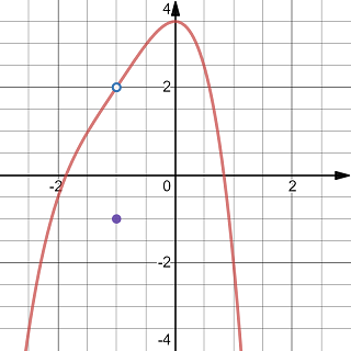
The graph of a function with a point replaced by another point

Solution.

When $x$ goes to $-1$, the point $(x, g(x))$ on the graph goes to the empty dot whose $y$-coordinate is 2. So the limit $\lim\limits_{x\to -1}g(x)=2$

Exercise 1.4 Evaluate the limit $\lim\limits_{x\to 1}f(x)$ using the graph of the function $y=f(x)$ shown in the figure.

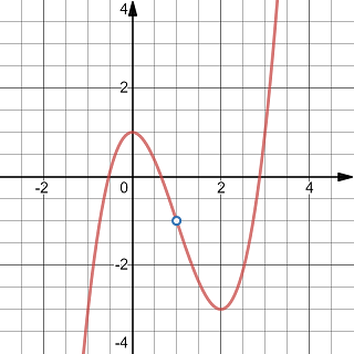
The graph of a function with a point removed

Solution.

When $x$ goes to $1$, the point $(x, f(x))$ on the graph goes to the empty dot whose $y$-coordinate is -1. So the limit $\lim\limits_{x\to 1}f(x)=-1$

Exercise 1.5 Use a table of functional values to evaluate \[ \lim\limits_{x\to 3}\frac{|x^2-9|}{x-3}. \]

Solution.

To estimate the limit, we evaluate the function $f(x)=\dfrac{|x^2-9|}{x-3}$ at some points that are close to $3$, for example, $x=3-0.01$, $3-0.001$, $3-0.0001$, $3+0.0001$, $3+0.001$, $3+0.01$. The function values can be seen in the following table.

$x$	$f(x)$	$x$	$f(x)$
3-0.01	-5.99	3+0.01	6.01
3-0.001	-5.999	3+0.001	6.001
3-0.0001	-5.9999	3+0.0001	6.001

From the table we see that

\[ -6=\lim\limits_{x\to 3^-}\frac{|x^2-9|}{x-3}\neq \lim\limits_{x\to 3^+}\frac{|x^2-9|}{x-3}=6. \]

So the limit $\lim\limits_{x\to 3}\frac{|x^2-9|}{x-3}$ does not exist.

Exercise 1.6 Use a table of functional values to evaluate \[ \lim\limits_{x\to 0}\frac{\cos x - 1}{x}. \]

Solution.

From the following table,

$x$	$f(x)$	$x$	$f(x)$
-0.01	0.00499996	0.01	-0.00499996
-0.001	0.0005	0.001	-0.0005
-0.0001	0.00005	0.0001	-0.00005

we estimate that \[ \lim\limits_{x\to 0}\frac{\cos x - 1}{x}=0. \]

Exercise 1.7 Consider the piece-wisely defined function \[ f(x)=\begin{cases} x-1 & {\text { if } x<1} \\ {x^{2}+1} & {\text { if } x\ge 1 }. \end{cases} \]

Evaluate the limits $\lim\limits_{x\to 1^-}f(x)$ and $\lim\limits_{x\to 1^+}f(x)$.
Determine if the limit $\lim\limits_{x\to 1}f(x)$ exists. Evaluate the limit if it exists. Otherwise, explain why it does not exist.

Solution.

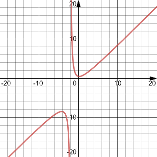
Using a calculator or a software, we may graph the function. A part of the graph of the function is shown in the following figure (which is created using desmos).

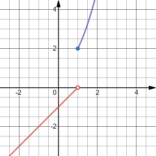
The graph of a piecewise function

From the graph, we see that $\lim\limits_{x\to 1^-}f(x)=0$ and $\lim\limits_{x\to 1^+}f(x)=2$.

So the limit $\lim\limits_{x\to 1}f(x)$ does not exist.

Exercise 1.8 Determine if the limit $\lim\limits_{x\to -1}\dfrac{|x+1|}{x+1}$ exists. Evaluate the limit if it exists. Otherwise, explain why it does not exist.

Solution.

From the graph of the function show below, we see that the left-limit and the right-limit do not agree. So the limit $\lim\limits_{x\to -1}\dfrac{|x+1|}{x+1}$ does not exist.

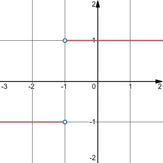
The graph of a function involve absolute value

Exercise 1.9 Determine the limit \[ \lim_{x\to -2^-}\frac{x^2+1}{x+2} \qquad\text{and}\qquad \lim_{x\to -2^+}\frac{x^2+1}{x+2}. \]

Solution.

As $x$ goes to $-2$, $x^2+1$ goes to $5$ and $x+2$ goes to $0$. The limits go to either infinity or negative infinity.

When $x<-2$, $x+2<0$ and $\frac{x^2+1}{x+2}<0$. So $\lim_{x\to -2^-}\frac{x^2+1}{x+2}=-\infty$.

When $x>-2$, $x+2>0$ and $\frac{x^2+1}{x+2}>0$. So $\lim_{x\to -2^-}\frac{x^2+1}{x+2}=\infty$.

This can also be seen by graphing the function.

The graph of a function with infinite limits at x=-2

Exercise 1.10 Determine the limit \[ \lim_{x \to -1^{+}} \frac{x^{2}+x}{x^{2}-x-2} \]

Solution.

We note that the rational expression can be simplified and the limit equals \[ \lim_{x \to -1^{+}} \frac{x^{2}+x}{x^{2}-x-2}=\lim_{x\to-1^{+}}\frac{x}{x-2}. \]

Since $\frac{x}{x-2}$ goes to $\frac{-1}{-1-2}=\frac13$ as $x$ goes to $-1$ from the right, the value of the limit is \[ \lim_{x \to -1^{+}} \frac{x^{2}+x}{x^{2}-x-2}=\frac13. \]

1.3 The Limit Laws

Theorem 1.1 (Basic Limit Results) For a constant number $c$, given a real number $a$, we have \[ \lim_{x\to a} c=c \qquad\text{and}\qquad \lim_{x\to a} x =a. \]

Theorem 1.2 (The Limit Laws) Suppose that the limits \[ \lim_{x\to a}f(x)\qquad \text{and} \qquad \lim_{x\to a} g(x) \] exists.
1. Sum: \[ \lim_{x\to a}(f(x)+g(x))=\lim_{x\to a}f(x)+\lim_{x\to a}g(x). \] 2. Scalar Multiplication: For any constant $c$, \[ \lim_{x\to a}(cf(x))=c\lim_{x\to a}f(x). \] 3. Product: \[ \lim_{x\to a}(f(x)g(x))=\lim_{x\to a}f(x)\lim_{x\to a}g(x). \] 4. Quotient: Suppose $\lim\limits_{x\to a}g(x)\neq0$. \[ \lim_{x\to a}\dfrac{f(x)}{g(x)}=\dfrac{\lim\limits_{x\to a}f(x)}{\lim\limits_{x\to a}g(x)}. \] 5. Power: For a positive integer $n$, \[ \lim_{x\to a}(f(x))^n=(\lim\limits_{x\to a}f(x))^n. \] 6. Radical: For a positive integer $n$, assume $\lim\limits_{x\to a}f(x)\geq 0$ if $n$ is even, \[ \lim_{x\to a}(\sqrt[n]{f(x)}=\sqrt[n]{\lim\limits_{x\to a}f(x)}. \]

Theorem 1.3 (Substitution Theorem) Let $P(x)$ and $Q(x)$ be polynomials. Suppose that $Q(a)\neq 0$. Then \[ \lim\limits_{x\to a}\frac{P(x)}{Q(x)}=\frac{P(a)}{Q(a)}. \]

Theorem 1.4 (Squeeze Theorem) Suppose that the functions $f$ and $g$ are defined and $f(x)\leq h(x) \leq g(x)$ holds on an interval $(a, c)\cup(c, b)$. If \[ \lim_{x\to c} f(x)=\lim_{x\to c}g(x)=L, \] then \[ \lim\limits_{x\to c}h(x)=L. \] Note: The value $c$ may be a finite number, $-\infty$, or $\infty$. The quantity $L$ may be a finite number, $-\infty$, or $\infty$ too.

Applying the squeeze theorem with $-|f(x)|\leq f(x)\leq |f(x)|$, we get the following corollary.

Corollary 1.1 Suppose that $\lim\limits_{x\to a}|f(x)|=0$. Then $\lim\limits_{x\to a} f(x)=0$.

An important limit which can be obtained by using the squeeze theorem is the following one. \[ \lim\limits_{x\to 0}\frac{\sin x}{x}=1. \]

Exercise 1.11 Evaluate the limit \[ \lim_{x\to -2}\frac{2x^2-1}{x^3+2x^2+1}. \]

Solution.

Since $(-2)^3+2(-2)^2+1=1\neq 0$, the limit can be evaluated by plugging in $x=-2$. We get \[ \lim_{x\to -2}\frac{2x^2-1}{x^3+2x^2+1}=\frac{2(-2)^2-1}{(-2)^3+2(-2)^2+1}=7. \]

Exercise 1.12 Evaluate the limit \[ \lim_{x\to 3}(2x-1)\sqrt{x+1}. \]

Solution.

Since $3+1=4$, the limit can be evaluated by plugging in $x=3$. We get \[ \lim_{x\to 3}(2x-1)\sqrt{x+1}=\frac{2(3)-1}{(3)+1}=\frac54. \]

Exercise 1.13 Evaluate the limit \[ \lim _{t \to 2}\left(\frac{t^{2}-2}{t^{3}-3t+5}\right)^{2} \]

Solution.

By plugging in $t=2$, we get \[ \lim _{t \to 2}\frac{t^{2}-2}{t^{3}-3t+5}=\frac{2^2-2}{2^3-3\cdot 2+5}=\frac27. \]

Applying the power rule, we get \[ \lim _{t \to 2}\left(\frac{t^{2}-2}{t^{3}-3t+5}\right)^{2}=\left(\frac27\right)=\frac{4}{49}. \]

Exercise 1.14 Evaluate the limit \[ \lim_{h\to 0}\frac{\sqrt{2x+h}-\sqrt{2x}}{h}. \]

Solution.

We cannot evaluate the limit directly by plugging in $h=0$. Because the denominator will be $0$. However, you may notice that the plugging-in trick can be applied after rationalizing the numerator. Here is how to do that. \[ \begin{aligned} &\lim_{h\to 0}\frac{\sqrt{2x+h}-\sqrt{2x}}{h}\\ =&\lim_{h\to 0}\frac{(\sqrt{2x+h}-\sqrt{2x})(\sqrt{2x+h}+\sqrt{2x})}{h(\sqrt{2x+h}+\sqrt{2x})}\\ =&\lim_{h\to 0}\frac{1}{\sqrt{2x+h}+\sqrt{2x}}\\ =&\frac{1}{2\sqrt{x}}. \end{aligned} \]

Exercise 1.15 Evaluate the limit \[ \lim_{t\to 0}\left(\frac{1}{t\sqrt{1+t}}-\frac{1}{t}\right). \]

Solution.

Since directly plugging in $t=0$ does not work, we evaluate the limit by first do some algebraic operations (simplifying and rationalizing the numerator). \[ \begin{aligned} &\lim_{t\to 0}\left(\frac{1}{t \sqrt{1+t}}-\frac{1}{t}\right)\\ =&\lim_{t\to 0}\left(\frac{1-\sqrt{1+t}}{t \sqrt{1+t}}\right)\\ =&\lim_{t\to 0}\left(\frac{-1}{(1+\sqrt{t+1})\sqrt{1+t}}\right)\\ =&-\frac{1}{2} \end{aligned} \]

Exercise 1.16 Evaluate the limit \[ \lim_{x\to 2}\left(\frac{3}{x^2-x-2}-\frac1{x-2}\right) \]

Solution.

We first simplify and then evaluate by plugging in. \[ \begin{aligned} &\lim_{x\to 2}\left(\frac{3}{x^2-x-2}-\frac1{x-2}\right)\\ =&\lim_{x\to 2}\left(\frac{3-(x+1)}{x^2-x-2}\right)\\ =&\lim_{x\to 2}\left(\frac{2-x}{x^2-x-2}\right)\\ =&\lim_{x\to 2}\left(\frac{-1}{x+1}\right)\\ =&-\frac13. \end{aligned} \]

Exercise 1.17 Evaluate the limit \[ \lim\limits_{x\to 0}x^2\cos\left(\frac1x\right). \]

Solution. Because $x^2\\ ge 0$ and $-1\leq \cos\left(\frac1x\right)\leq 1$. We see that \[ -x^2\leq x^2\cos\left(\frac1x\right)\leq x^2. \] Note that $\lim\limits_{x\to 0}(-x^2)=0$ and $\lim\limits_{x\to 0}x^2=0$. By the squeeze theorem, \[ \lim\limits_{x\to 0}x^2\cos\left(\frac1x\right)=0. \]

Exercise 1.18 Evaluate the limit \[ \lim\limits_{x\to 0}\frac{1-\sin x}{|x|}. \]

Solution.

Note that $1\leq 1-\sin x\leq 2$ and $|x|>0$ for $x\neq 0$. Therefore \[ \frac1{|x|}\leq \frac{1-\sin x}{|x|} \leq \frac2{|x|}. \]

Because $\lim\limits_{x\to 0}\frac{1}{|x|}=\lim\limits_{x\to 0}\frac{2}{|x|}=\infty$. Then \[ \lim\limits_{x\to 0}\frac{1-\sin x}{x}=\infty. \]

Exercise 1.19 Evaluate the limit \[ \lim\limits_{x\to 0}\left((x+1)^2-\frac{\sin x}{x}\right). \]

Solution. s

Since $\lim\limits_{x\to 0}\frac{\sin x}{x}=1$ and $\lim\limits_{x\to 0}(x+1)^2=(0+1)^2=1$. By the sum rule, \[ \begin{aligned} &\lim\limits_{x\to 0}\left((x+1)^2-\frac{\sin x}{x}\right)\\ =&\lim\limits_{x\to 0}(x+1)^2- \lim\limits_{x\to 0}\frac{\sin x}{x}\\ =&1-1=0. \end{aligned} \]

Exercise 1.20 Suppose $\lim\limits_{x\to 0}|f(x)|=0$. Evaluate the limit \[ \lim\limits_{x\to 0}\frac{(f(x)-1)^2}{x^2+2}. \]

Solution.

Point-wisely, $-|f(x)|\leq f(x)\leq |f(x)$. Then by the squeeze theorem and the given assumption $\lim\limits_{x\to 0}|f(x)|=0$, we can conclude that \[ \lim\limits_{x\to 0}f(x)=0. \]

By limit laws, we find that \[ \lim\limits_{x\to 0}\frac{(f(x)-1)^2}{x^2+2} =\frac{(\lim\limits_{x\to 0}f(x)-1)^2}{\lim\limits_{x\to 0}(x^2+2)} =\frac{(-1)^2}{0^2+2} =\frac12. \]

1.4 Continuity

Intuitively, a function is continuous means that there is no holes or jumps when moving on the graph of the function.

Definition 1.1 A function $f$ is continuous at $x=a$ if \[ \lim_{x\to a}f(x)=f(a). \]

Note that the equality requires three true statement to hold.

The function $f$ is well-defined at $a$, that is $a$ is in the domain of $f$.
The limit $\lim\limits_{x\to a}f(x)$ exists as a finite number.
The limit equals the value $f(a)$ of the function.

If $f$ is defined near $a$ but $f$ is not continuous at $a$, we say that $f$ is discontinuous at $a$.

The discontinuity is called a jumping discontinuity if the one-side limits exist but have different values.

A discontinuity is called a removable discontinuity if the limit exists.

A discontinuity is called an infinite discontinuity if a one-side limit is the infinity or the negative infinity.

Note that we may also define continuous from the left or the right using one-side limits.

A function $f$ is continuous on an interval if it is continuous at every number in the interval, where at an endpoint of the interval, we understand continuity as from the left or the right.).

Derived from limit laws, we have the following theorem for continuity.

Theorem 1.5 Suppose that two function $f$ and $g$ are continuous at $a$. For a constant number $c$, the sum $f+g$, the scalar multiplication $cf$, the product $f\cdot g$, and the quotient $\frac{f}{g}$ (given that $g(a)\neq 0$) are all continuous at $a$.

As a corollary to the direct substitution theorem, we know that all polynomial and rational functions are continuous over their domain.

Indeed, it can be proved that root functions and trigonometric functions are also continuous at every number in their domains.

One important operation for producing new functions is the composition. For continuous functions, as you may expect, continuity works well with composition.

Theorem 1.6 Let $f$ be a function continuous at $c$ and $g$ be a function continuous at $f(c)$. Then $f\circ g$ is continuous at $c$.

A slightly more general result is the following.

Theorem 1.7 Let $f(x)$ be a function continuous at $L$ and $g$ be a function such that $\lim\limits_{x\to c}g(x)=L$. Then \[ \lim\limits_{x\to c}f(g(x))=f(L). \]

Continuous functions have many important (actually fundamental) properties. One of them, which has been used in the test-point method to solve inequalities in some algebra books, is call the intermediate value theorem.

Theorem 1.8 (Intermediate Value Theorem) Let $f$ be a function continuous on the interval $[a, b]$. If $f(a)\cdot f(b)<0$, then there exists a number $c\in (a,b)$ such that $f(c)=0$.

Exercise 1.21 Find the domain of the function \[ f(x)=\frac{x-1}{x^2+1} \] and use definition of continuity and limit laws to determine whether the function is continuous over its domain.

Solution.

Since $x^2+1>0$, the domain of the function is $(-\infty, \infty)$. By limit laws, for any number $a$, \[ \lim_{x\to a}f(x)=\lim_{x\to a}\frac{x-1}{x^2+1}=\frac{a-1}{a^2+1}=f(a). \] So the function is continuous over $(-\infty, \infty)$.

Exercise 1.22 Find the domain of the function \[ f(x)= \begin{cases} \frac{x^2-2x-3}{x-3} & x\neq 3\\ 4 & x=3. \end{cases} \] Use definition of continuity and limit laws to determine whether the function is continuous over its domain.

Solution.

The domain of the function is $(-\infty, \infty)$. When $x\neq 3$, the function is a rational function and hence continuous at any where except $x=3$. By limit laws, \[ \lim_{x\to 3}f(x)=\lim_{x\to 3}\frac{x^2-2x-3}{x-3}=\lim_{x\to 3}(x+1)=4=f(3). \] So the function is continuous over $(-\infty, \infty)$.

Exercise 1.23 Find the domain of the function \[ f(x)= \begin{cases} x^2+1 & x<0\\ 1 & x=0 \\ \frac{\sin x}{x} & x>0. \end{cases} \] Use definition of continuity and limit laws to determine whether the function is continuous over its domain.

Solution.

The domain of the function is $(-\infty, \infty)$. By properties of continuous functions, the function is continuous except possibly at $x=0$. When $x=0$, the left and right limits are \[ \lim_{x\to 0^-}f(x)=\lim_{x\to 0^-}(x^2+1)=1 \quad \text{and} \quad \lim_{x\to 0^+}f(x)=\lim_{x\to 0^+}\frac{\sin x}{x}=1. \] It follows that \[ \lim_{x\to 0}f(x)=1=f(0). \] So the function is continuous over $(-\infty, \infty)$.

Exercise 1.24 Find the discontinuity and determine its type for the function \[ f(x)=\frac{|x|}{x}. \]

Solution.

Removing the absolute sign, the function can be written as \[ f(x)= \begin{cases} 1 & x>0\\ -1 & x<0 \end{cases} \] So the function has a discontinuity at $x=0$. It’s a jumping discontinuity because \[ \lim\limits_{x\to 0^-}f(x)=-1\neq 1=\lim\limits_{x\to 0^+}f(x). \]

Exercise 1.25 Find the discontinuity and determine its type for the function \[ f(x)=\frac{2x^2-x-3}{x+1}. \]

Solution.

This function is a rational function which is undefined only at $x=-1#. So a possible discontinuity is at $x=-1$. To determine the type, we find the limit first. \[ \lim\limits_{x\to 1}f(x)=\lim\limits_{x\to 1}\frac{2x^2-x-3}{x+1}=\lim\limits_{x\to 1}(2x-3)=-1. \] So the function has a removable discontinuity at $x=-1$.

Exercise 1.26 Evaluate the limit \[ \lim_{x\to 2} (x-1)^2\sqrt{13-x^{2}}. \]

Solution.

Since products and compositions of continuous functions are continuous, using properties of continuous functions, we have \[ \lim_{x\to 2} (x-1)^2\sqrt{13-x^{2}}=(2-1)^2\sqrt{13-2^{2}}=4. \]

Exercise 1.27 Evaluate the limit \[ \lim_{x\to \frac{\pi}{2}} \sin(x-\cos(x)). \]

Solution.

Since products and compositions of continuous functions are continuous, using properties of continuous functions, we have \[ \lim_{x\to \frac{\pi}{2}} \sin(x-\cos(x))=\sin\left(\frac{\pi}{2}-\cos\left(\frac{\pi}{2}\right)\right)=1. \]

Exercise 1.28 Find the value of the constant $c$ such that the function \[ f(x)=\begin{cases} c x^{3}+3 & \text { if } x<1 \\ x^{2}-c x & \text { if } x \ge 1 \end{cases} \] is continuous over $(-\infty,\infty)$.

Solution.

The function is only possibly discontinuous at $x=1$. To make the function continuous at $x=1$, we first need the existence of the limit. Since \[ \lim_{x\to 1^-} f(x)=c+3 \quad \text{and} \quad \lim_{x\to 1^+} f(x)=1-c. \]
The limit of $f$ exists at $x=1$ if and only if $c+3=1-c$. Solve for $c$, we get $c=-1$ and $\lim\limits_{x\to 1}f(x)=2$. Hence $f(1)=\lim\limits_{x\to 1}f(x)=2$.

So the function is continuous over $(-\infty,\infty)$ if $c=-1$.

Exercise 1.29 Suppose $f$ and $g$ are continuous functions over $(-\infty,\infty)$ such that $f(2)=1$, $g(2)=4$ and $f(4)=3$. Find the limit \[ \lim\limits_{x\to 2} \frac{f(g(x))+\sqrt{g(x)}}{2f(x)g(x)-1} \]

Solution.

Because $f$, $g$ and the function $y=\sqrt{x}$ are continuous. The composite functions $f(g(x))$ and $\sqrt{g(x)}$ are continuous. By arithmetic rules and the definition of continuous functions, we have note that \[ y=\frac{f(g(x))+\sqrt{g(x)}}{2f(x)g(x)-1} \] is a continuous function too. Therefore, \[ \lim\limits_{x\to 2} \frac{f(g(x))+\sqrt{g(x)}}{2f(x)g(x)-1} =\frac{f(g(2))+\sqrt{g(2)}}{2f(2)g(2)-1} =\frac{f(4)+\sqrt{4}}{2\cdot 1\cdot 4-1} =\frac57. \]

Exercise 1.30 Use the Intermediate Value Theorem to show that the equation \[ x^3-\cos(x)-1=0 \] has a root in the interval (0, 2).

Solution.

Let $f(x)=x^3-\cos(x)-1$. As a linear combination of continuous functions, $f$ is also continuous. Note that \[ f(0)f(2)=(0-\cos 0 -1)(2^3-\cos 2-1)=-2\cdot(7-\cos2)<0. \]

The IVT theorem tells us that there exists a number $c\in(0,2)$ such that $f(c)=0$. So the equation has a solution $x=c$ in $(0,2)$.